Getting started
Install
There are three ways in, and the downloads page describes each in full.
A compiled package — nothing to set up: download, open, and the application is on your desktop. Builds for macOS (Apple silicon and Intel, signed and notarised), a Windows installer and a Linux AppImage. This is the one to take unless you already work in Python.
The Python package — the desktop application and the scripting API are one package, so installing it gets you both: the analysis you can drive from a notebook, and the same window the installers put on your desktop.
(On PyPI from the first release; until then the name is held by an empty placeholder.)
A contributor install — take the repository and install it in place, so your edits are live without reinstalling:
Python 3.12 or newer, whichever way. The dependencies come with the
package: numpy, scipy, pandas, h5py, netCDF4, pint, vtk, pyvista,
pyvistaqt, PySide6, pyqtgraph, openpyxl. One is optional: the
STEP/IGES importer's geometry kernel, which the compiled packages
include and a Python install adds with
pip install "visualdynamics[step]".
The app
visualdynamics-gui                  # or: python -m visualdynamics
visualdynamics-gui modal_run.nc4    # opening files on the way in
A compiled package opens like any other application; the commands above are for the Python install.
Every launch of this alpha opens with a disclaimer to acknowledge — the software is offered as is, its numbers are the user's to check — and File → About Visual Dynamics… shows the version, readable without the network.
File → Check for Updates… asks visualdynamics.org whether a newer version exists and says so — up to date, newer (with the download page to open), or unreachable. It never downloads or replaces anything itself: a newer version is installed the way the first one was.
The command is created by the install, in the environment's own bin
directory — it is on your PATH exactly when that environment is
active. From a terminal that has not activated it, either activate
first or call it by path; both run the same thing:
Drag files anywhere onto the window to import them: Rattlesnake runs
(.nc4), universal files (.unv/.uff), I-DEAS ADFs
(.afu/.ati/.ash), Exodus meshes (.exo), Nastran bulk decks
(.bdf/.dat/.nas) and punch eigenvectors (.pch), Femap Neutral
files (.neu), sdynpy arrays (.npz/.npy), channel-table
spreadsheets (.xlsx), CAD geometry (.step/.iges tessellated on
import — a McMaster-Carr download drops straight in — and .3mf or
.stl meshes, each part a named block),
photographs, and whole .vdyn projects. The
full matrix of what each format carries, both directions, is in
Importing and exporting.
Launching from a session that uses sdynpy
import sdynpy binds pyqtgraph to PyQt5 and sets QT_API=pyqt5, and
neither can be undone once a process has started — so a notebook or
VS Code session that has been using sdynpy cannot host visualdynamics's window
in that same interpreter. visualdynamics.launch_gui() notices and starts the
app in a fresh process instead, returning immediately:
import sdynpy, visualdynamics
visualdynamics.launch_gui('modal.vdyn')     # its own process; sdynpy is untouched
Pass in_process=True to insist on this interpreter (and get the
explanation if it cannot work), or in_process=False to always use a
separate one — handy in a notebook, where the window then does not
block the kernel.
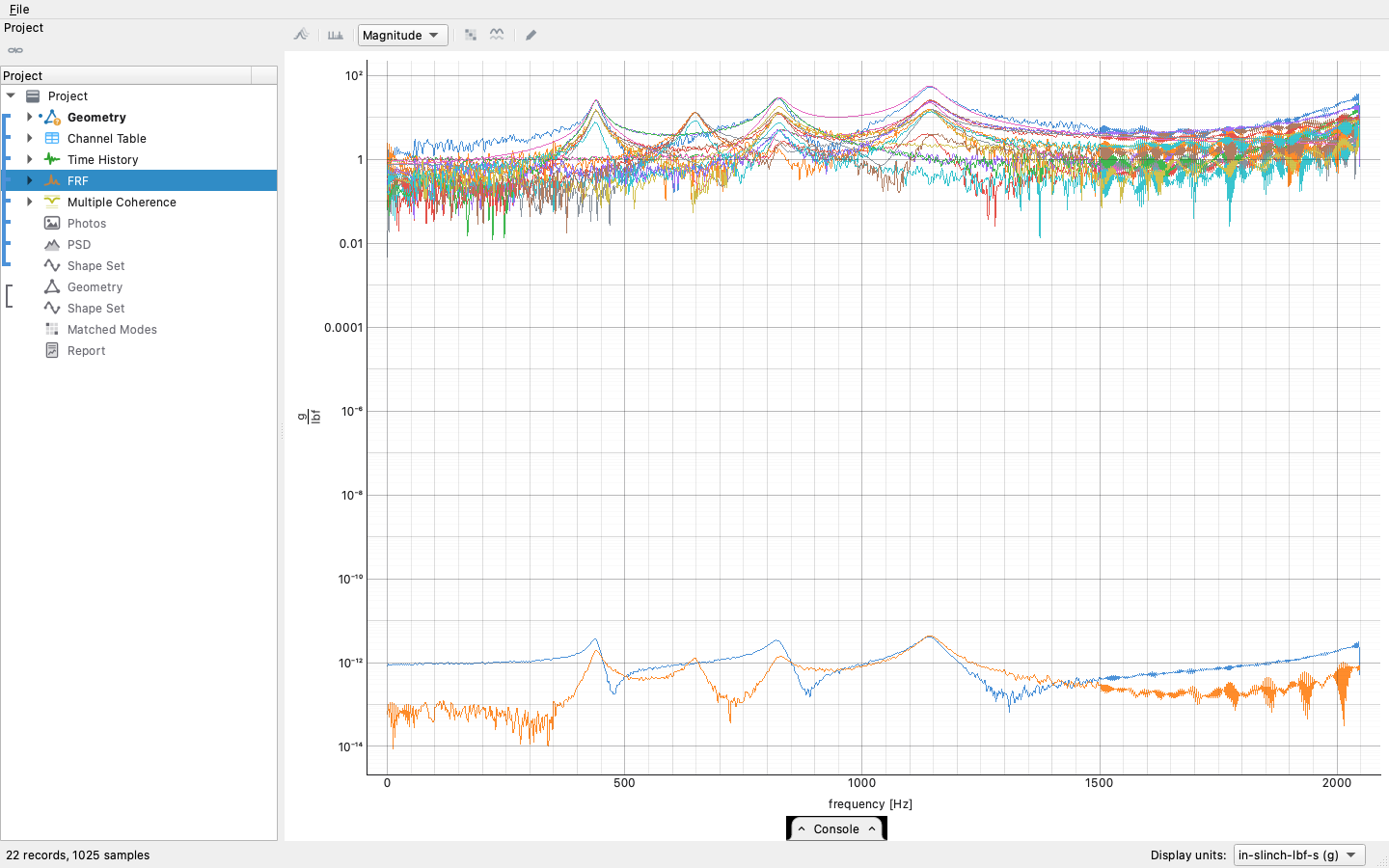
Drag files onto the project tree to import them. Right-click the project root to set its type; select two objects and use the link bar to declare they belong together. Computations live where their settings are set: a time history's averaging view carries the spectral estimates (Compute PSDs, CPSDs, FRFs, Multiple Coherence, Spectra), the shock view carries Compute SRS, and the filter and truncate views apply their own acts — each panel's buttons compute with exactly the settings on screen. The transforms with no view of their own (integrate, differentiate, extract sine levels, the modal fit) are acts on the same bar — an icon each, the verb in its tooltip, offered only for the selection they apply to; with the project row selected the bar holds Generate Report. Objects copy and paste like files — Cmd/Ctrl-C and V in the tree duplicates them, pasting into a folder exports them, and a copy from another window carries them across. When a settings change leaves a derived object behind — more averages on the time data, a moved shock window — a refresh badge appears beside it saying why, and clicking the badge recomputes it in place.
The same thing as a script
import visualdynamics

project = visualdynamics.Project('Beam Airplane Modal Test')
project.project_type = 'Modal Test'
project.import_file('modal_run.nc4')
project.import_file('test_geometry.npz')
project.geometry.define_units('m')
project.set_basis(*list(project))       # the measured side

project.compute_psds(project.basis.time_history)
project.fit_modes(project.basis.frf, bounds=(5.0, 120.0))

project.basis.frf.plot()                # the app's own plot, in a window
project.save('modal.vdyn')              # open this in the app
examples/modal_workflow.py in the repository is a longer version of
this — import, process, fit, correlate, match, plot, report — and it
runs as a test, so it always works.
Which one should I use?
Both, in either order. The app is faster for looking, judging and picking; a script is faster for repeating. They share the objects, the rules and the file, so a project can move between them mid-job: save from the app, load in a notebook, save again, reopen.
The one thing a script cannot do is the judgement calls the screen asks you for — which residual peak is a real mode, which MAC squares are a match. Scripted, those become rules (a frequency band, a MAC threshold), and it is worth being deliberate about that.
And the bridge between the two is built in: the console tab along the bottom of the window writes the session as Python while you work — every import, every setting, every computation as the line that replays it, judgement calls included (an interactive mode fit journals as its confirmed picks). Expand the tab, copy the stretch you want, and yesterday's session is today's script.