The sine sweep workflow

A sine test drives the article at a tone — or several at once — and walks each tone along its own schedule. The specification is not a band to fill but a trajectory to hold: this frequency at this time at this level, with warning and abort tolerances around it. So the questions the workflow answers are a sweep's own: did each tone hold its level, everywhere along its path?

The walkthrough is the demonstration plate's sweep — four simultaneous tones on four shakers into eight control channels, each tone on its own schedule: one sweeping up, one down through it, a near-dwell, and a log sweep — 16.5 seconds at 4096 Hz. The recording is generated by the controller (generate_plate_sine.py in the generators repository) and lands at stressdata/plate/sine.nc4.

Step	In the app	In a script
Import the run	drag the .nc4 onto the window	project.import_file(path)
The specification	arrives with the run — nothing to declare	(read from the file's environment)
See the sweep itself	the time history's wavelet reading	plot_scalogram(...) from visualdynamics.plot
Extract the levels	Extract Sine Levels on the bar	project.extract_sine(project.time_history)
Judge them	select levels and specification together	plot_comparison(levels, spec) from visualdynamics.plot
Geometry and photos	drag them in, link them	project.add(...), project.link(...)
Report	Generate Report on the bar, the project row selected	project.generate_report('sine')
Save	Save Project As…	project.save('sine.vdyn')

In the app, step by step

1. Import the run — the specification comes with it

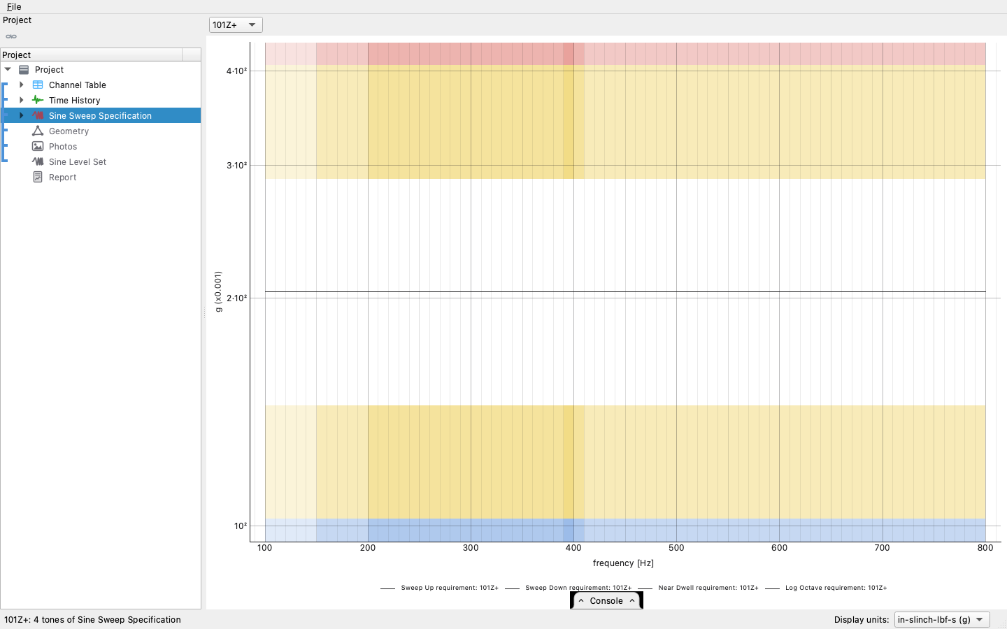
Drag the controller's recording onto the window. Unlike a shock or a transient, a sine run can say what it is: the file's environment carries the tones' schedules, so the project arrives typed Sine Sweep with its specification already in the tree — each tone's frequency trajectory, its target level along it, and the warning and abort bands around that. Selecting the specification opens on the stage — frequency across, time receding, amplitude up, one surface per tone — and the 3-D toggle stands it down to the flat per-channel reading shown here; picking rows in the grid below restricts either reading to the tones picked.

2. See the sweep itself

Before any number is extracted, the record can be looked at the way a sweep actually is: the time history's wavelet reading draws frequency against time with amplitude as colour, and a multi-tone sweep is its natural subject — four tones are four ridges, each walking its own path, crossing where they cross. The spectra a random workflow leans on would average all of that away.

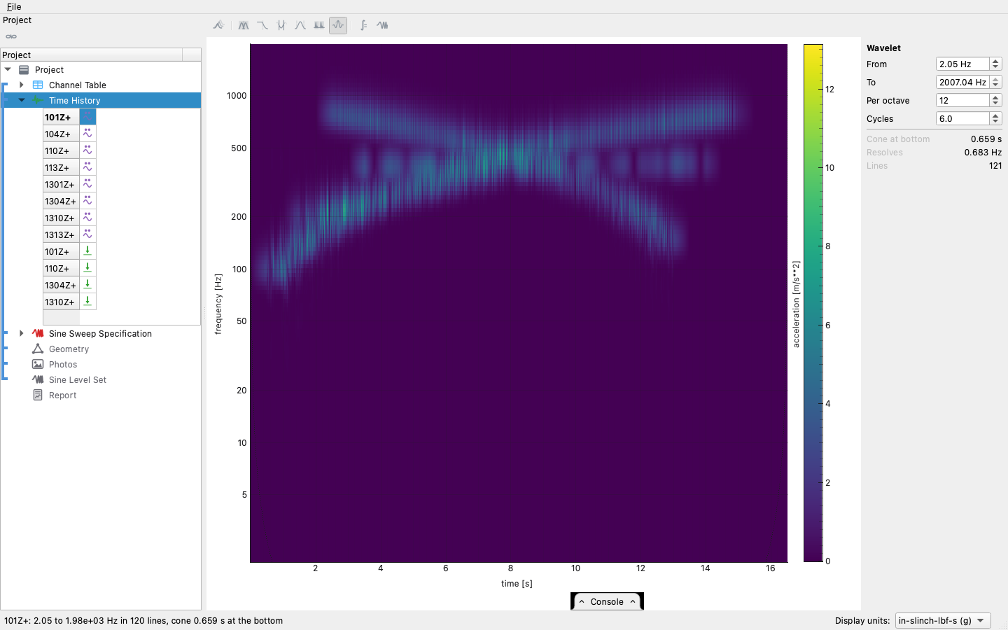
The ribbed look along each ridge is the record, not the transform: tones that pass within a wavelet's bandwidth of each other beat at their difference frequency, and the modulation is genuinely in the measured signal — band-pass the record with no wavelet anywhere and the same ripple is there.

3. Extract the levels

Extract Sine Levels on the bar, with the time history selected, reads each tone's achieved level out of the recording with a Vold-Kalman filter: every tone's own frequency trajectory is rebuilt from the specification, and the amplitudes riding all of them are solved for at once, each held to a slow curve over a set number of cycles. That is what separates the reading from a PSD — a swept tone never sits still long enough for an average — and, because the tones are solved jointly, two tones that run close together for a stretch are separated by their different frequency histories rather than each reading the other as its own level, which is what a tracking filter (the controller's own included) does.

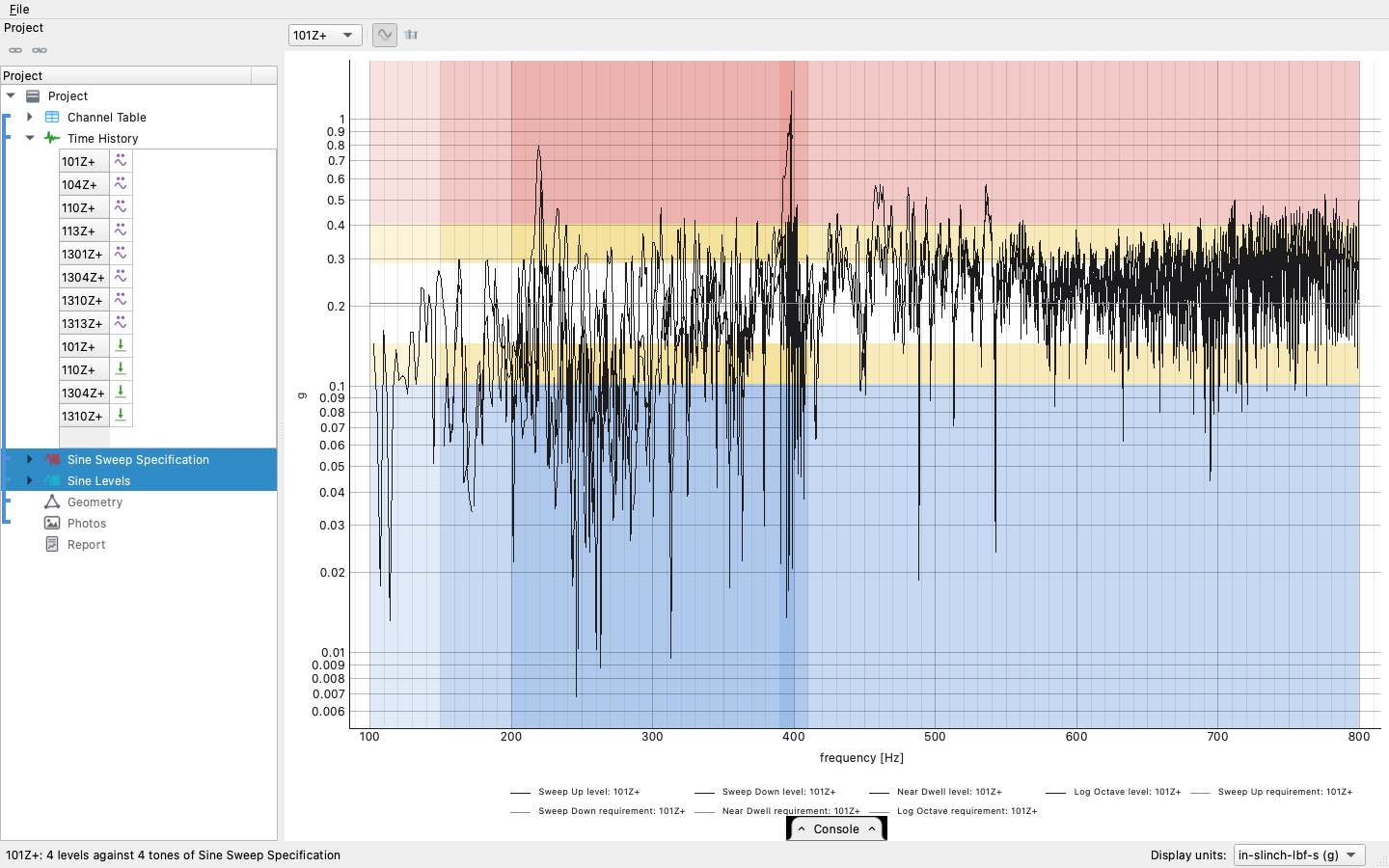
One object comes out, grouped the way the specification groups its tones, with a per-tone clock. Selecting the levels beside the specification draws each measured path over its target and zones, clocks aligned — on the stage by default, flat with the 3-D toggle off; the signed deviation bars judge the whole run tone by tone.

4. Geometry, photos, report

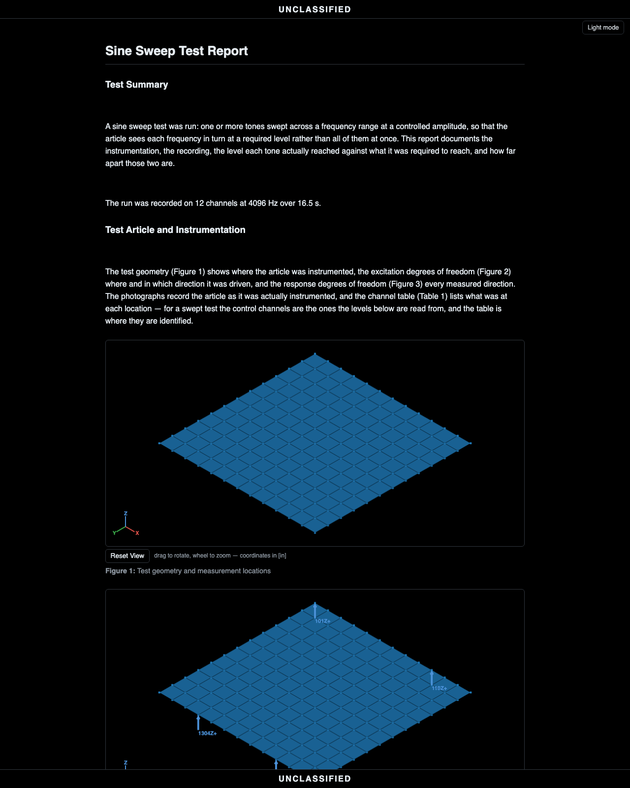
Drag the article's geometry in, declare its units, add the setup photographs, link the group. The sine report binds the specification, the levels over it, and one figure per tone — each tone judged along its own path, which is the only way a sweep can honestly be judged.

The same run, headless

And the script never has to be reconstructed by hand: the console tab along the bottom of the window writes it live as you click — every act of the session as the line that replays it. Expand it, copy the stretch you want, and it runs as-is.

import visualdynamics

project = visualdynamics.Project('Plate Sine Sweep')

# 1. the run carries its own specification; the project arrives typed
project.import_file('sine.nc4')
assert project.project_type == 'Sine Sweep'

# 2. geometry, photos, links
geometry = visualdynamics.import_file('geometry.npz')
geometry.define_units('m')
project.add('Geometry', geometry)
project.link(*project.names)
project.set_basis(*project.names)

# 3. the levels each tone actually held, solved jointly (Vold-Kalman)
project.extract_sine(project.time_history)

# 4. report and save
project.generate_report('sine')
project.export_report(project.report, 'sine_report.html')
project.save('sine.vdyn')

Where judgement lives

• A mixed run imports both specifications. A random environment over a quiet sweep — the qualification-with-a-tracked-tone case — arrives with the random specification leading and the sine one beside it, and each is judged by its own workflow. Which specification the run was for is the engineer's call, not the file's.
• The extraction is per-tone, not per-band. Each tone is read along its own trajectory, and all of them together, so two tones crossing — or running close for seconds — do not corrupt each other's levels the way any fixed filter bank, or a tracking filter, would. What the extractor cannot do is separate two tones that share a trajectory — a tone and its own harmonic landing on another tone's path is read as that tone.
• Where the levels wobble, look at the wavelet first. A ripple in an extracted level can be the article (a resonance walked through), the test (two tones beating in one band), or the extraction. The scalogram shows which: a resonance is a bright patch at a fixed frequency, beating is ribbing where ridges pass close, and neither is the extractor's fault.
• Ramp time is part of the trajectory. A tone leaves its start frequency at start_time + ramp_time, and the extracted clock is aligned to the tone's onset — a lead-in before the sweep starts is not a level error, and the comparison does not read it as one.