How a PSD means its area¶

A power spectral density is not a curve that happens to have an area — the area is the measurement. The RMS of the signal is the square root of the area under its PSD, a specification's overall level is the area under its breakpoints, and octave banding is nothing but the same area rearranged. So Visual Dynamics treats "how is a value read between the points" as one fact per object, interpolation, and both the integral and the picture come from it. A spectrum drawn one way and integrated another is a picture of a number nobody computed — which is not hypothetical: the PSD of a transient target was once drawn as a power law through four thousand density lines while its level was worked out as their area, and the field exists so that cannot happen again.

There are two readings, and every figure below is drawn by the same call the application uses (tools/make_concept_figures.py regenerates them).

'bin' — constant across its own bin¶

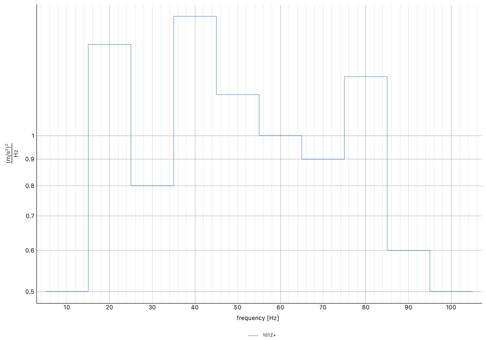
A computed PSD is a density per analysis bin: each line's value holds flat across its bin, the area is the sum of value times width, and it draws as steps. For a narrowband spectrum the bins are the midpoints between neighbours — inferring them is exact. This example's ten coarse lines have values summing to 10 over 10 Hz bins, so the area is exactly 100 (m/s²)² and the RMS is exactly 10 m/s² — and the steps are that sum, visibly.

Ten narrowband lines drawn as steps: each value flat across its
midpoint-to-midpoint bin, the edges landing half a bin beyond the
first and last lines

The same power on octave bands¶

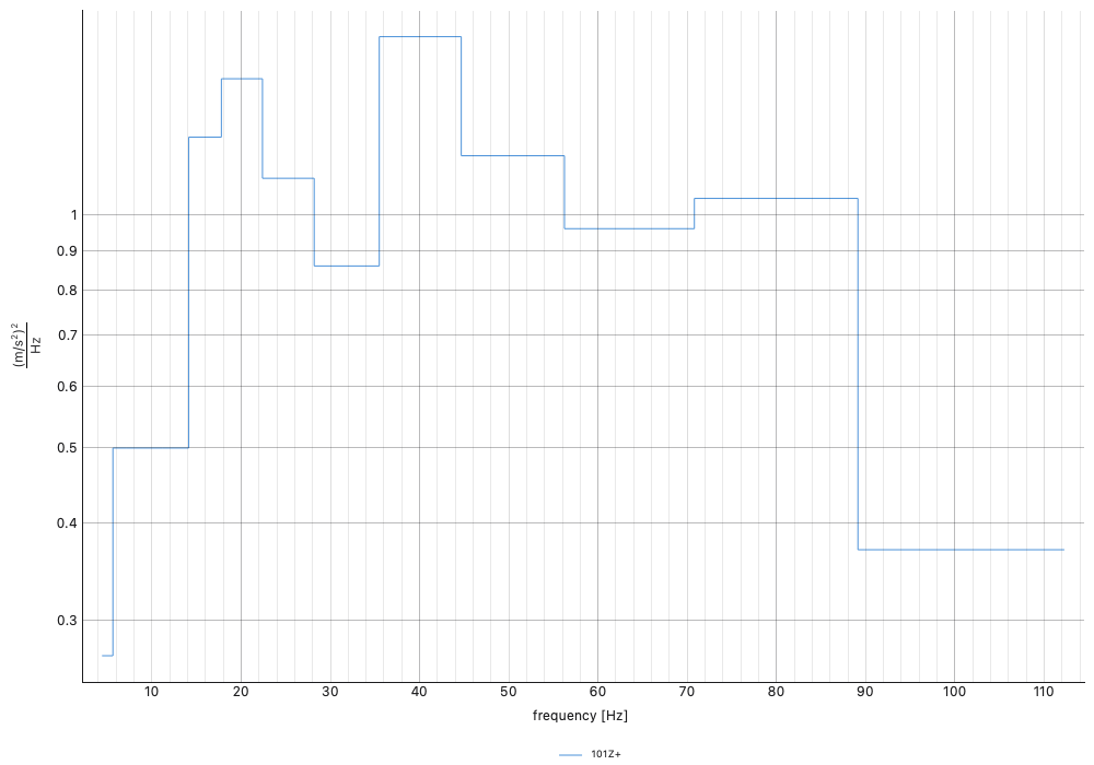
Banding onto proportional bands (the plot bar's Octave Bands reading and its Apply Octave Bands button; project.compute_octave in a script) conserves the area — the same power, arranged the way it is read. An octave-band spectrum sets bandwidth, because its bins are geometric and its edges are a standard's, not its neighbours': reading them off the centres would be a hair out at every band and wrong at the two ends. The steps land on the standard's own edges, and the RMS is still exactly 10 m/s².

The same spectrum on third-octave bands: geometric bins on the
standard's edges, wider with frequency, holding the same
area

'log_log' — a power law between breakpoints¶

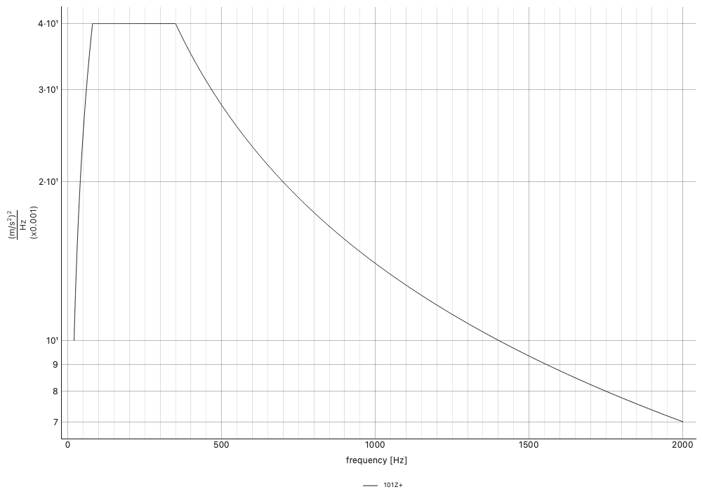
A specification written at a handful of breakpoints is a continuous requirement: between breakpoints it is the straight line the two points make on log-log axes, which is a power law, and its area has a closed form. It draws as that curve — on the linear frequency axis below the power-law segments show their true curvature — and its area() integrates the same law, 6.06 m/s² RMS for this one.

A four-breakpoint specification drawn as the power law it is: flat
top, rising and falling power-law skirts

The reading is per instance, not per class: a specification authored at a dozen breakpoints is a curve, but a specification computed from a record — a transient target's PSD — is a density like any other, and carries 'bin'.

Checking it¶

psd.area()                  # the one integral, read as drawn
psd.area(low=20.0, high=2000.0)      # over a band
rms = psd.area() ** 0.5

banded = psd.to_octave(6)   # sixth octaves, conserving the area
assert abs(banded.area() - psd.area()) < 1e-9 * psd.area()

There is deliberately no second integral to reach for: whichever way a spectrum is read, area() reads it the same way it is drawn, and nothing outside the object chooses.

In the window, a specification on its own opens as its spectra. RMS on the plot bar is the other reading: a bar per channel of the level it asks for — the root of that same area — with the table of the numbers beneath, and nothing coloured, since a specification alone has nothing to be out of. Records picked in the tree restrict both. A specification with a measurement beside it has the comparison's three readings instead.