The shock workflow

A shock test names a response spectrum: the article must see an event whose SRS lands inside a tolerance band around the required curve, and the waveform that does it is the machine's business. So the report leads with the transients — a shock's whole character is in the trace — and answers the narrower spectral question after.

The walkthrough is the demonstration plate's shock series — four half-sine events walked up to level, six accelerometers and a drive — photographed at every step. The recording ships with the repository (testdata/plate/shock.nc4).

Step	In the app	In a script
Import the recording	drag the .nc4 onto the window	project.import_file(path)
Say what it is for	right-click the root → Set Project Type → Shock	project.project_type = 'Shock'
The events	the time view marks each shock	(detected, or the record's own frames)
Compute the SRS	Compute SRS in the shock view	project.compute_srs('Time History')
The required SRS	import it, with its tolerance	visualdynamics.ShockSpecification(...)
Compare	select SRS and specification together	plot_comparison(srs, spec) from visualdynamics.plot
Geometry and photos	drag them in, link them	project.add(...), project.link(...)
Report	Generate Report on the bar, the project row selected	project.generate_report('shock')
Export	Export HTML…	project.export_report(name, path)
Save	Save Project As…	project.save('shock.vdyn')

In the app, step by step

1. Import the recording, and say what it was

Drag the machine's recording onto the window. A shock recording is indistinguishable from a transient at the file level — one stream of events — so the run arrives as Transient and the engineer declares it: right-click the project root and set the type to Shock. The tree grows the slots a shock report draws from. There is no coherence slot — a shock is one event, and coherence is a statement about a stationary average.

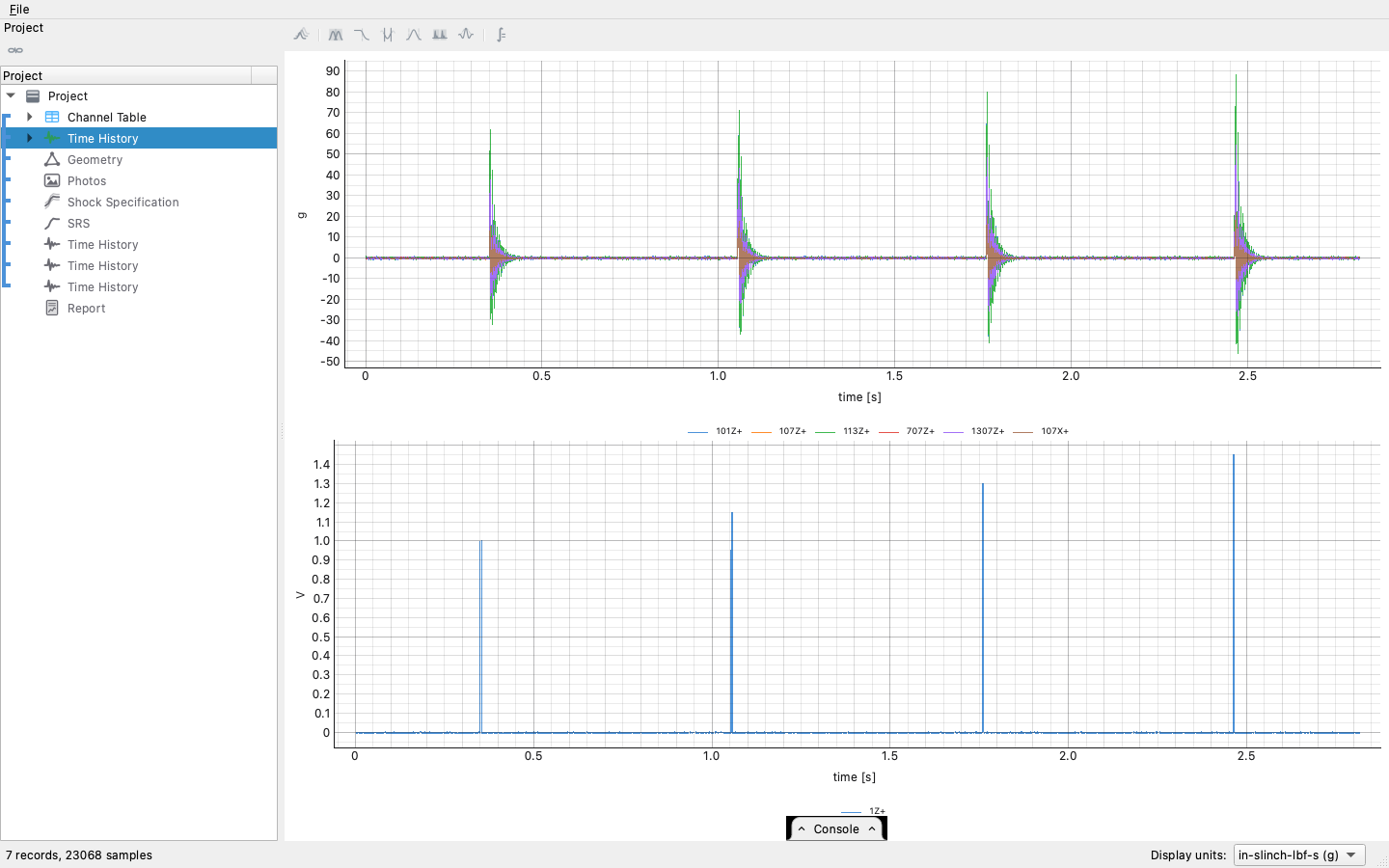
The events are found, not assumed: open the shock view and Detect finds them — an act you take, not a greeting the record opens with — and a record whose frames already say (a controller's save) keeps its own. The time view shades each found event on the trace. Detected windows share one length by default — the longest any event needs, peak to settled ringdown — because events windowed alike are compared alike; the Same length for all box on the panel releases them. Dragging a window's body moves that one event; dragging an edge resizes it, and under the shared length resizing one resizes the series, stopping before any window would swallow a neighbour.

2. Compute the shock response spectra

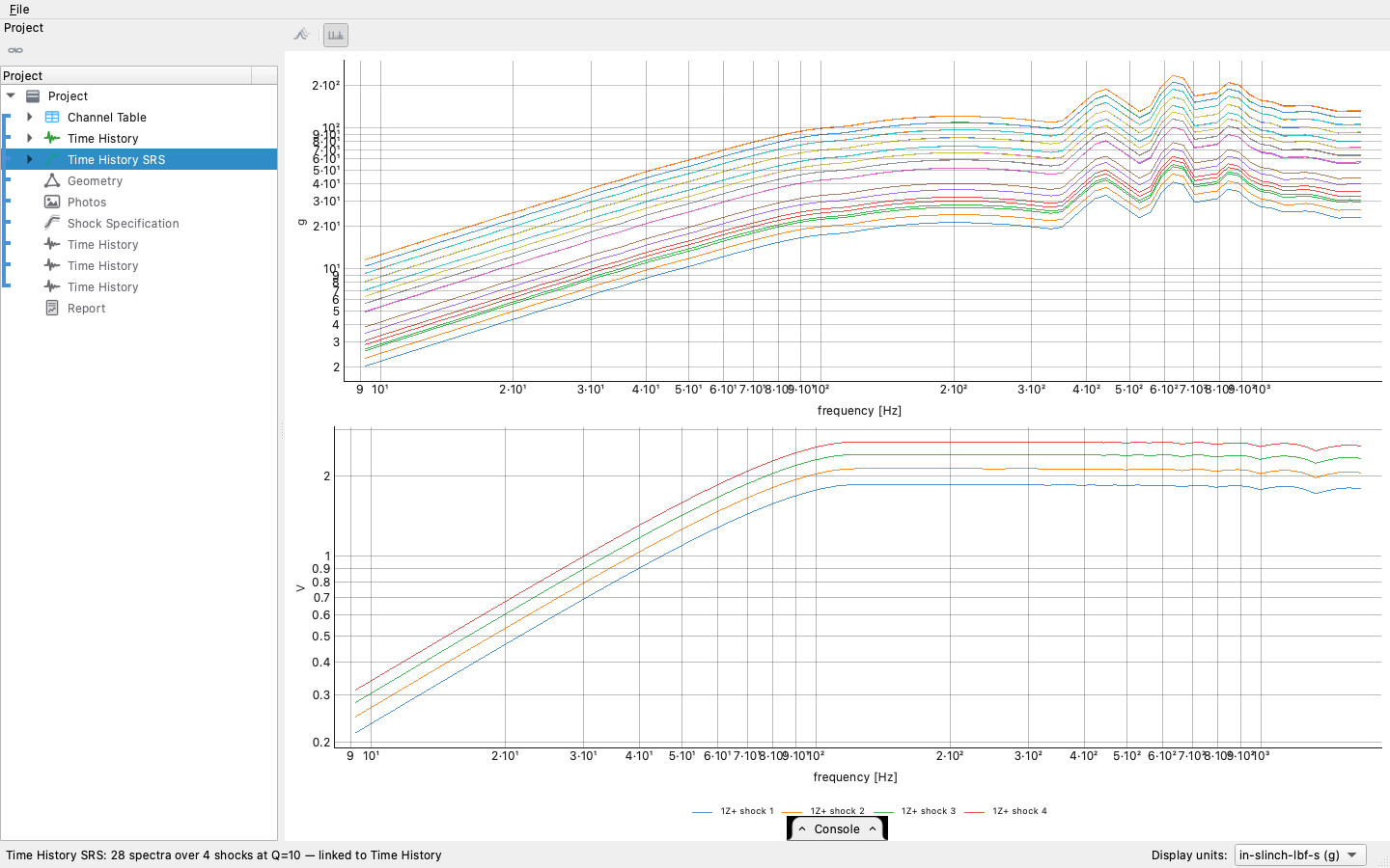
Compute SRS in the shock view — beside the windows it reads — computes one SRS per channel per event: a shock test is judged on the worst event, so a recording holding four has to answer as four, not as an average. (A whole-record spectrum is one window set over the whole record, which the view can say outright.) The plot shows every event at one channel: a walked-up series reads as a family of curves climbing to level, and the drop-down on the bar reaches the other channels.

3. The requirement, and the comparison

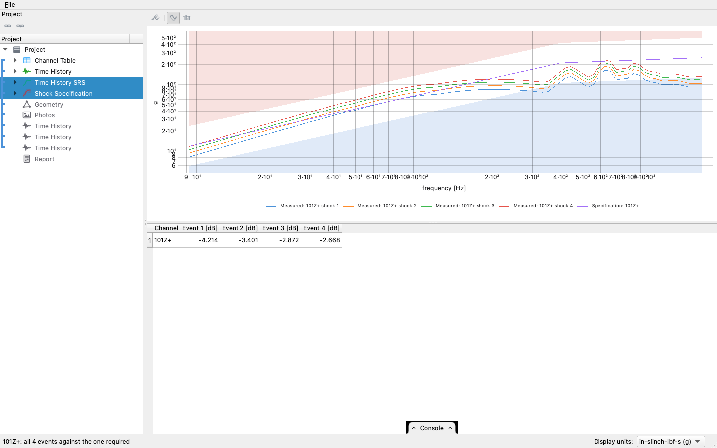
A shock specification is an SRS with room around it — the required curve with its tolerance band (abort_upper, abort_lower). Import it, or author it once in a script and save it. Selecting the measured SRS and the specification together shades the band around the spectra — still every event at one control channel — and the SRS Error view reads the whole run as bars: every event at every control channel, the RMS deviation from the requirement in decibels, signed — blue past −6 dB where the shock under-tested, red past +6 dB where it over-tested — exactly as the random workflow's RMS error bars read.

4. Geometry, photos, report

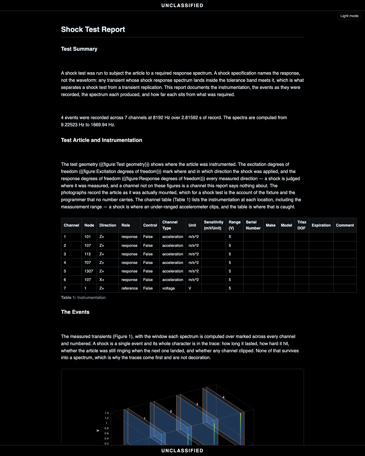
Drag the article's geometry in, declare its units, add the setup photographs, link the group. The shock report leads with the time histories, the detected windows shaded on them — how long, how many, whether the article was still ringing when the next event landed is in the trace and nowhere in the spectrum — then the specification with its band, the control channels' SRS drawn over it exactly as selecting both shows in the app, the signed deviation bars that judge it, and the scalogram of the filtered record: where in frequency each event's energy sat and when, which is what names the source of an unexpected SRS peak. (There is no PSD in a shock report: a density of a transient recording carries a level set by how much quiet air was captured, and the scalogram answers the frequency question with the time axis still attached.)

The same series, headless

And the script never has to be reconstructed by hand: the console tab along the bottom of the window writes it live as you click — every act of the session as the line that replays it. Expand it, copy the stretch you want, and it runs as-is.

import numpy as np

import visualdynamics
from visualdynamics.core.data import ShockSpecification

project = visualdynamics.Project('Plate Shock Series')

# 1. import, and declare what the file cannot say
project.import_file('shock.nc4')
project.project_type = 'Shock'

# 2. one SRS per channel per event; detection runs only because
# nothing else says where the events are
project.compute_srs(project.time_history)

# 3. the requirement: breakpoints with a tolerance band around them
srs = project.srs
frequencies = np.asarray(srs.abscissa, dtype=float)
level = ...                       # the required curve, from the test plan
project.add('Shock Specification', ShockSpecification(
    abscissa=frequencies, ordinate=level[None, :],
    response_dof=[srs.response_dof[0]],
    ordinate_dim='acceleration', ordinate_unit='m/s**2',
    q=srs.q, kind=srs.kind,
    abort_upper=level[None, :] * 10.0 ** 0.3,     # +6 dB: a factor of 2
    abort_lower=level[None, :] * 10.0 ** -0.3))   # -6 dB

# 4. geometry, photos, report
project.add('Geometry', visualdynamics.import_file('geometry.npz'))
project.geometry.define_units('m')
project.link(*project.names)
project.set_basis(*project.names)
project.generate_report('shock')
project.export_report(project.report, 'shock_report.html')
project.save('shock.vdyn')

Where judgement lives

• Which events count. The generator walked this series up to level, and a real one is walked up too: the report shows every event's spectrum, and which were qualification and which were rehearsal is the engineer's sentence to write.
• The tolerance itself. ±6 dB is the band the demo authors (+6 dB and −3 dB is the usual convention); a real specification carries its own band, and the shading in every comparison comes from the object rather than from a setting.
• Q, and what the spectrum means. An SRS is computed at one amplification — quoted at Q = 10, it says nothing about what the same shock does to a Q = 50 article — so the value travels with the spectrum and the specification alike, and comparing spectra at different Q is refused rather than fudged.
• The window length. Above a knee — a window long enough to hold the peak and its ringdown — the SRS barely moves with further length, which is what makes one shared length safe as the default. The judgement is whether a window reached the knee: a ringdown cut short reads low at the article's own frequencies, and the shaded windows on the trace are where to look.