The modal workflow

A modal test in, identified modes and a report out — done in the app, in a script, or half and half: the window holds the same Project a script builds, calling the same verbs, so a project built by clicking and one built by running code are the same project and each opens in the other.

The walkthrough below is one complete survey, photographed at every step — the demonstration plate's own modal test, a burst-random Rattlesnake run on two shakers. The same files ship with the repository (testdata/plate/), so every step here can be followed exactly.

The map first, then each path in full.

Step	In the app	In a script
Start a project	it starts empty	project = visualdynamics.Project('Name')
Import	drag files anywhere on the window	project.import_file(path)
Declare units	the Imported Units pane	obj.define_units('m')
Group what belongs together	select, then the link bar	project.link('Geometry', 'FRF', ...)
Name the measured side	right-click the bracket → Basis of Comparisons	project.set_basis(...)
PSDs from the captures	Compute PSDs in the averaging view	project.compute_psds('Time History')
Identify modes	the fitting screen: Find Mode, drag, Confirm Mode	project.fit_modes('FRF', bounds=(300, 1300), limit=5)
Correlate	select both shape sets — the MAC appears	project.comparison_mac('A', 'B'); project.plot_mac('A', 'B') draws it
Commit matches	pick squares, press +	project.match_modes('A', 'B', threshold=0.7)
Report	Generate Report on the bar, the project row selected	project.generate_report('modal')
Export	Export HTML…	project.export_report(name, path)
Save	Save Project As…	project.save('modal.vdyn')

In the app, step by step

1. Import the survey

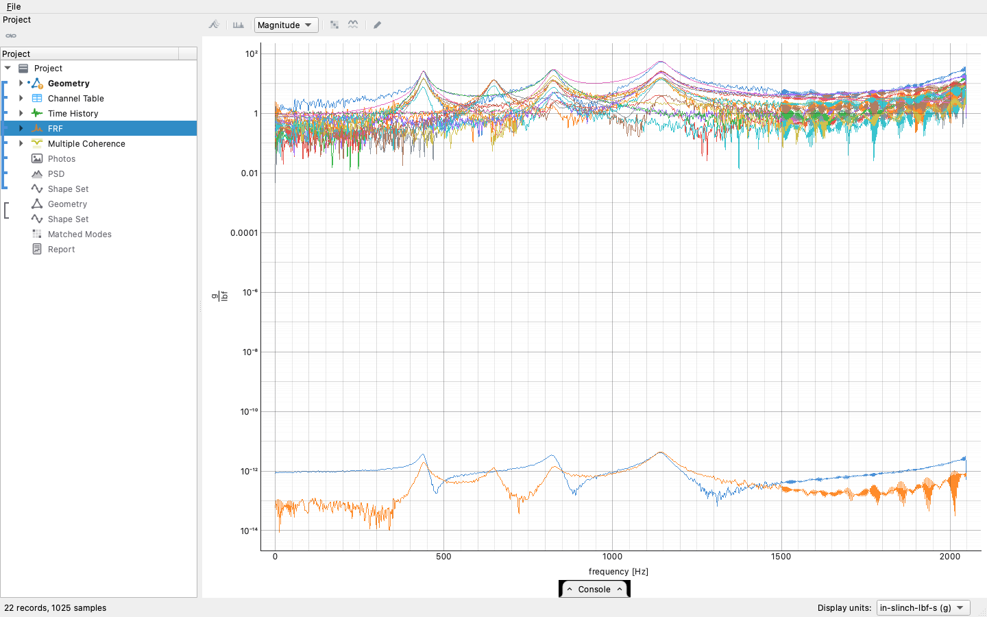
Drag the controller's spectra save and the test display geometry anywhere onto the window. The run says what it was — the project type switches to Modal Test by itself — and the tree grows grey slots for everything a modal report draws from. The slots are the to-do list: each disappears as the real object arrives.

2. Declare what the files did not say

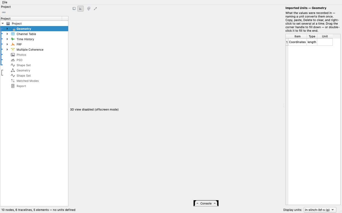
The controller's file carries its units, so its objects arrive defined. The geometry came from an .npz that says nothing, so it arrives raw — select it and give the Imported Units pane the one answer it asks for. Nothing is ever scaled by a guess: undefined objects wear a badge until a person answers.

The article's CAD can stand behind the survey too: a STEP, IGES, 3MF or STL file imports as face elements, one block per part, and sits in the same group as context.

3. Link the measured side, and call it the Basis

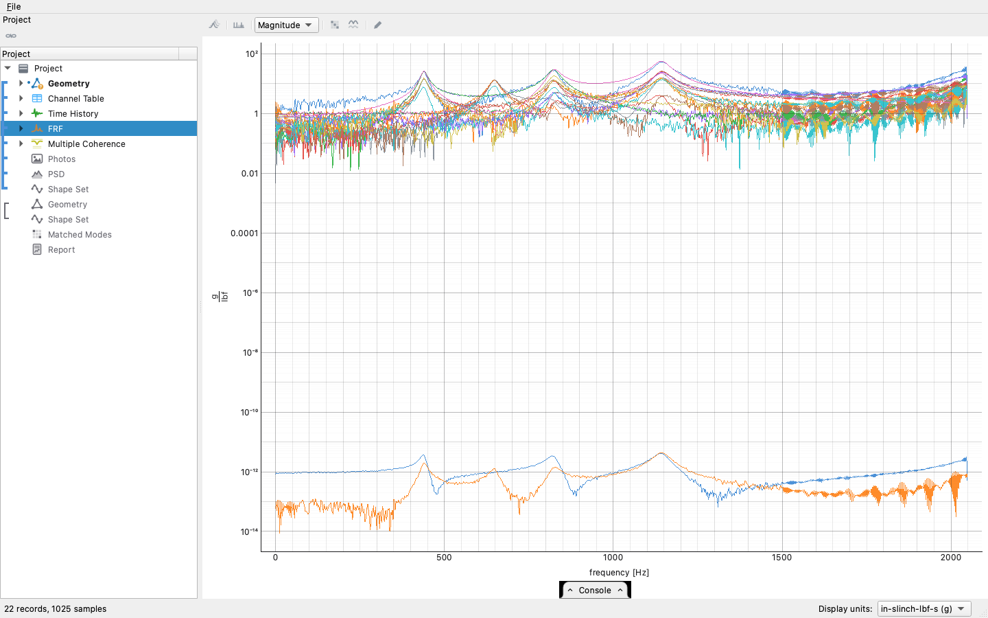
Select everything the test measured and link it; the bracket painted down the tree's left edge is the group. Right-click the bracket and tick Basis of Comparisons: comparisons happen in its DOFs, its modes make the MAC rows, and every @basis: binding in the report resolves through it.

4. PSDs from the captures

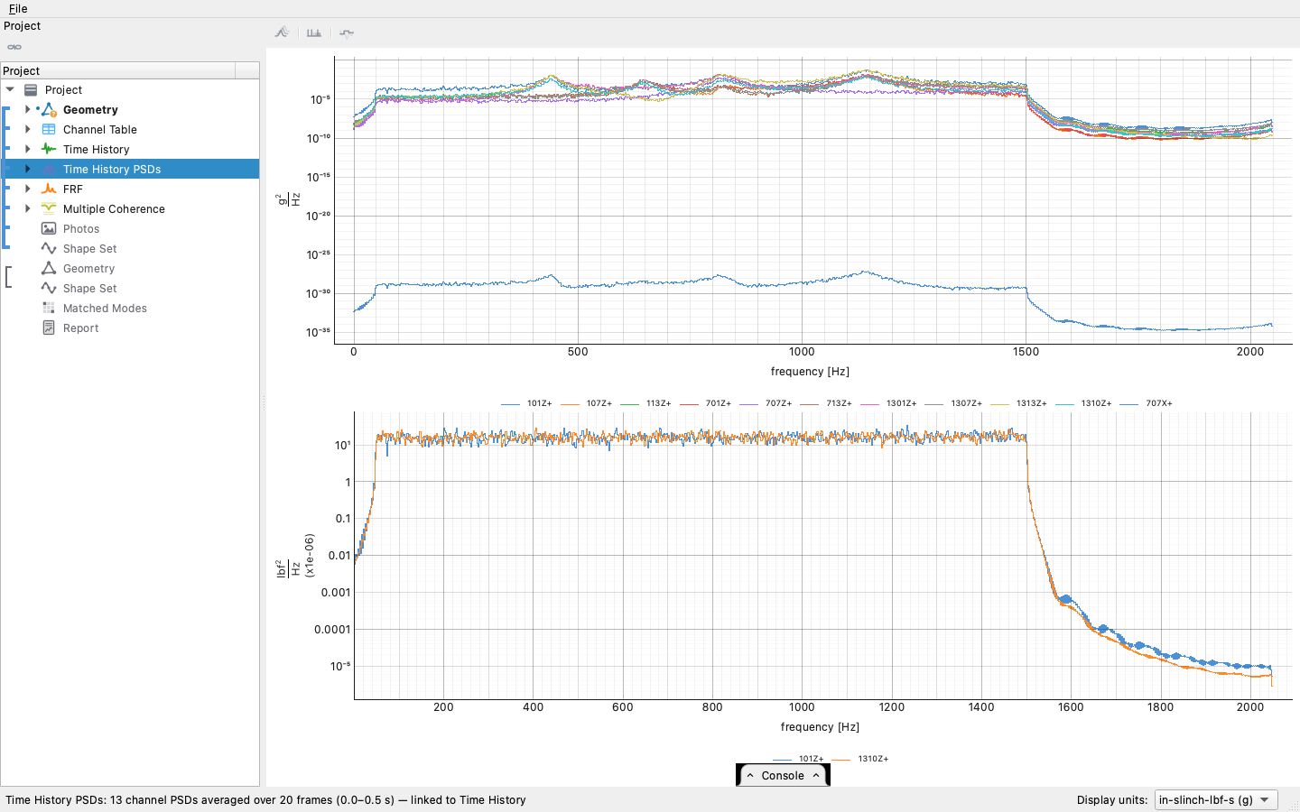
The time data is twenty burst captures, one per accepted average. Open the averaging view — it shows the captures one playing at a time, the pager stepping between them, and the panel counts what pools (20 × 1 = 20 averages) — and Compute PSDs: the densities are averaged over exactly those frames, the run's own averaging, not a guess, and land beside the record, linked into the group.

5. Identify modes on the fitting screen

Select the FRF and open the fit. The loop runs left to right along the bar: Find Mode puts the cursor on the most prominent CMIF peak left in the residual, the fit follows the cursor as you drag and settles when it stops — judge the dashed synthesis and the MAC — and Confirm Mode takes it and moves to the next peak. Once two modes are confirmed, Refine All appears at the left: a joint re-fit of every residue with all the modes present, for the pairs that lean on each other (fit_modes(..., refine=n) in a script).

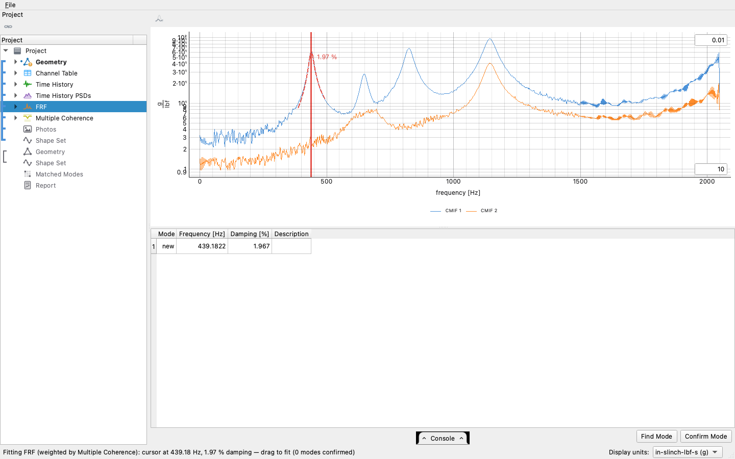
The cursor is two controls in one: left and right is frequency, and dragging vertically holds the damping — the dashed parabola under the cursor shows the mode about to be fitted, its width the damping made visible. The algorithm, and how it differs from the classical batch methods, is its own page: How the mode fitting works.

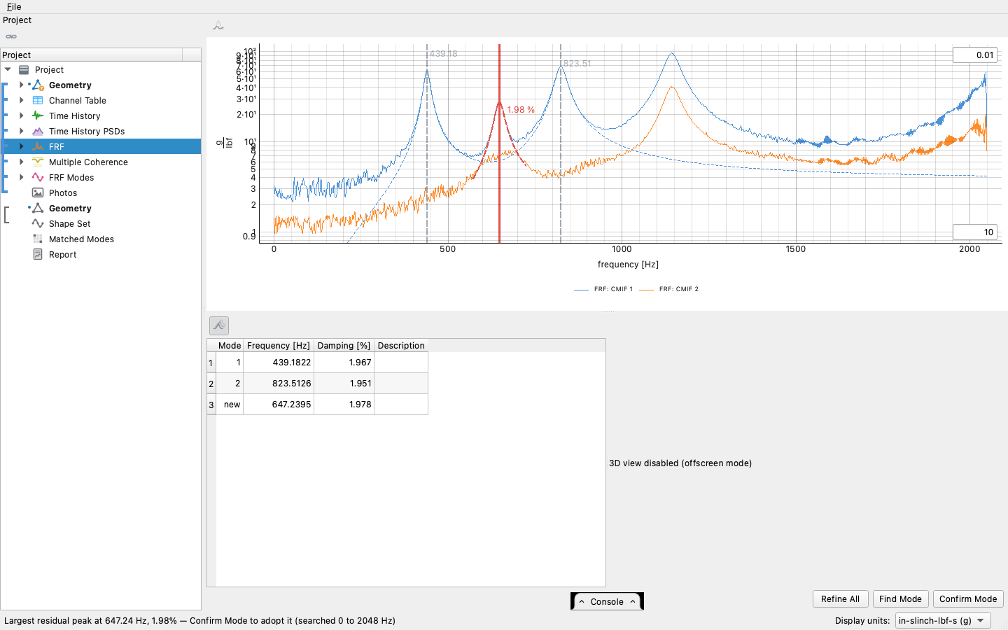
Five confirms take the plate's five modes in the band — four distinct peaks, and the repeated pair's second mode at 1142 Hz, which Find Mode reaches through the first tooth's shadow because the shape standing in the residual there is not the one already taken. The published shape set is the complete fit state: select it and choose Edit Fit later and the session reopens exactly where it stood.

6. Look at a shape

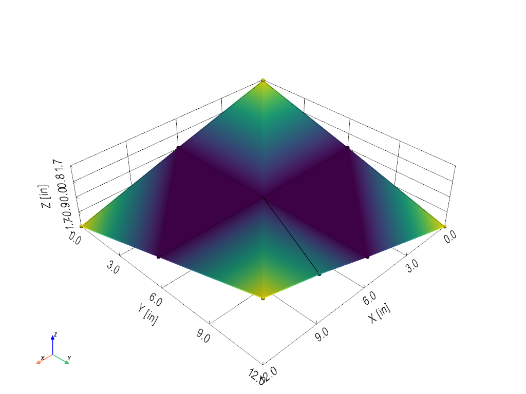
Select the fitted shape set beside its geometry and the modes animate on the survey panels, deflected and coloured by displacement.

7. Correlate against the model

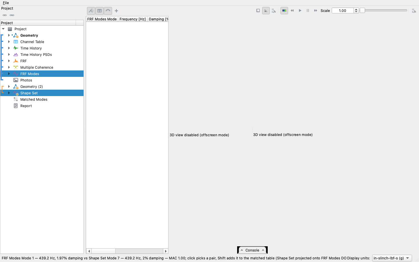
Import the FEM pair — the full meshed plate and its computed modes — declare their units, and link them as their own group. The pair can arrive as the solver's own files: a Nastran bulk deck (.bdf) for the mesh with a punch file (.pch) for the eigenvectors, a Femap Neutral (.neu) carrying both at once, or an Exodus mesh with sdynpy or UNV shapes — the interchange matrix has the full list. Select the two shape sets together and the cross-MAC appears, fitted modes across, FEM modes down. Clicking a square picks the pair and the status bar reads it back; Shift adds it to the matched table, and + commits the selection as a Matched Modes object.

8. Generate the report

Generate Report on the bar, with the project row selected, builds the modal report: every figure and table binds symbolically (@basis:Frf, not a name), so renaming objects later changes nothing. Fill in the prose blocks — test summary, conclusions — and Export HTML writes one self-contained file that opens in any browser.

The same survey, headless

And the script never has to be reconstructed by hand: the console tab along the bottom of the window writes it live as you click — every act of the session as the line that replays it. Expand it, copy the stretch you want, and it runs as-is.

The identical run of verbs, in order — the same sequence as examples/modal_workflow.py, which the test suite executes so it cannot drift, under the names this page uses. The step numbers match the walkthrough above.

import visualdynamics

project = visualdynamics.Project('Plate Modal Survey')
project.project_type = 'Modal Test'

# 1. import — the run switches the type and fills the first slots
project.import_file('modal_spectra.nc4')
project.import_file('test_geometry.npz')

# 2. declare what the files did not say
project.geometry.define_units('m')

# 3. the measured side is the basis
project.set_basis(*project.names)

# 4. PSDs over the run's own captures
project.compute_psds(project.basis.time_history)

# 5. identify the five modes in the band
project.fit_modes(project.basis.frf, bounds=(300.0, 1300.0),
                  limit=5, name='Identified Modes')

# 7. the FEM pair, and the matches
project.add('FEM Geometry', visualdynamics.import_file('geometry.npz'))
project.add('FEM Shapes', visualdynamics.import_file('shapes.npy'))
project.link('FEM Geometry', 'FEM Shapes')
project.other.geometry.define_units('m')
project.other.shapes.define_units('kg')
project.match_modes(project.basis.shapes, project.other.shapes,
                    threshold=0.7)

# 8. report, export, save
project.generate_report('modal')
project.export_report(project.report, 'modal_report.html')
project.save('modal.vdyn')            # opens in the app as-is

Every plot the app draws has a call, and path= (scenes: screenshot=) renders it headless — step 6's figure is one line:

basis = project.basis
basis.frf.plot_cmif(basis.shapes, path='cmif.png')
project.plot_mac(basis.shapes, project.other.shapes, path='crossmac.png')
project.animate(basis.shapes, mode=0, screenshot='mode1.png')

Where judgement lives

Two steps ask you to look and decide:

• Which peaks are modes. The fitting screen shows the residual CMIF; you confirm a mode and watch what is left. Scripted, fit_modes confirms the most prominent residual peak and stops at limit — the plate's demo caps at five, because eleven channels cannot honestly distinguish more in that band, and left uncapped the loop will dredge the noise floor. A rule that stands in for the eye, and worth checking against the CMIF. And the judgement, once made, travels: an interactive session journals to the console as fit_modes(at=[(frequency, damping), ...]) — the confirmed picks themselves, in the order taken — so the fit you shaped by eye replays exactly in a script.
• Which MAC squares are matches. Clicking picks them. Scripted, match_modes takes each mode's best partner above a MAC threshold, or an explicit list of pairs.

Everything else — importing, converting, computing, correlating, reporting — is the same code either way.

Scaling, and when it is real

A modal fit splits residues into shape coefficients only when a drive point was measured: a response at the excitation DOF. Visual Dynamics does that automatically when the data has one — the plate survey measures both of its shaker points for exactly this reason. Without one, the scale is a convention: frequencies, damping, shapes and MAC are all fine, but modal masses are not physical, and the set says so — in the status bar, in the mode table's column heading, and in the report's parameter table caption.