How a tracking filter reads a sweep¶

A swept-sine controller does not measure the response the way Extract Sine Levels does. It reads the response at the drive frequency through a tracking filter, a band-pass centered on the drive frequency that follows it along the sweep, and it turns what comes out into a level with a detector. Both are settings, and the same response record gives a different level curve for each. When a controller's level and an extracted one disagree, the reason is usually in those two settings, and visualdynamics.core.sine_tracking reads a record each way so the difference can be seen.

The band and the detector¶

The band has a fixed width in Hz, or a width proportional to the drive frequency, as a fraction of it. A common setting on the test floor is proportional, around half the drive frequency; the ranges offered run from a few percent to the whole drive frequency proportional, or from about one hertz to several hundred fixed. With no band, the detector reads the record as it stands.

The detector is one of four:

Detector	`detector=`	Reads	Reported as
Filter output	`'filtered'`	the band's own output amplitude, at the instant	itself
Peak	`'peak'`	the largest absolute sample over the last cycle	itself
RMS	`'rms'`	the root mean square over the last cycle	times √2
Mean	`'mean'`	the mean absolute value over the last cycle	times π/2

The last two are reported as the peak of the sine they would be, so for a clean tone all four read its amplitude. For anything else they differ, and that is the point.

What a harmonic does¶

A clipped amplifier drive puts a third harmonic on the response. Read without a filter, a peak detector counts the harmonic's peaks: a harmonic of 30 % in phase with its tone reads 30 % high. An RMS detector counts its power instead: the same harmonic reads √(1 + 0.3²), about 4.4 % high. Through the band, neither is seen: the harmonic sits at three times the drive frequency, outside any band narrower than four times the drive. (A mean detector on the same record reads about 10 % low: the harmonic in phase sharpens the peaks and hollows the shoulders, and the shoulders hold more of the area.) Broadband noise behaves the same way: an unfiltered RMS reading counts all of its power, and a band counts its own share.

A 10 m/s² log sweep with a 30 % third harmonic, read four ways: the
unfiltered peak at 13, the unfiltered RMS at about 10.4, and both
filtered readings on the specification at
10

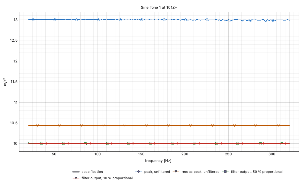
What the band costs¶

A band takes time to follow a change in level, roughly one over its width. A level that doubles part way through a sweep is followed in a millisecond by an unfiltered peak detector, in 9 ms through a 50 % band at 250 Hz, in 37 ms through a 10 % band, and in 180 ms through a 5 Hz fixed band (the time to reach half way, in each case). On a sweep at 100 Hz/s, 180 ms is 18 Hz of the frequency axis, read low. The fourth-order filter also overshoots a step by about a tenth of it before it settles.

A linear sweep whose level doubles at 250 Hz, read through bands of
different widths: the wide band follows the step at once, the 5 Hz
fixed band lags it by tens of hertz and
overshoots

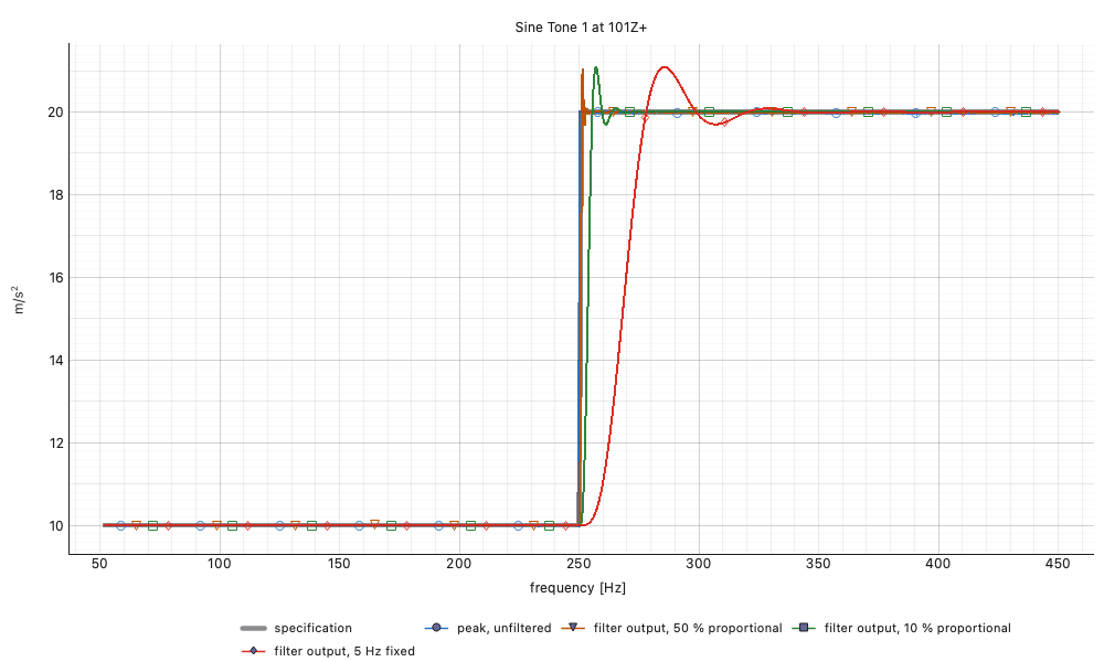
So the trade is settling time against rejection: a narrow band holds out harmonics and noise and lags a change in level, such as a resonance passed through quickly; a wide band follows the change and counts more of what is not the tone.

Seeing the band on the record¶

A level curve says what the band read and hides why. The band is easier to understand drawn where it was applied, so plot_tracking_filter draws one setting on one tone of the record:

The record and what the band passes, the record in gray and the band's output over it in magenta. The tone comes out of the harmonic and the noise at its own amplitude, sample by sample.
The record's scalogram, time across and frequency up a log axis, colored in dB below its loudest point so the noise floor is visible, with the cone of influence veiled as in the wavelet guide. Over it, the band is drawn as a corridor that follows the sweep: two dashed lines at the drive frequency plus and minus half the bandwidth, the band's −3 dB edges. The tone runs up the middle of the corridor, the third harmonic runs parallel to it outside, and the noise fills the rest of the picture.
The band's shape at a cursor, beside the picture on the same frequency axis: its magnitude in dB, with the drive marked inside the band by a circle and the harmonic outside it by a triangle. A readout gives the drive frequency, the band's edges, the settling time (one over the bandwidth) and how far down the band holds the harmonic.
The band's weight on the record, shaded behind the cursor. The band's output at an instant is the record before that instant, weighted by the filter's impulse response, so the shading shows how far back the reading reaches. That distance is the settling time.

A proportional band is a constant width on the log axis, so its corridor runs parallel to the tone. A fixed band is a constant width in hertz, so its corridor is wide at the bottom of the axis and narrows toward the top. At 100 Hz the 50 % band is 75 to 125 Hz, settles in about 20 ms and holds the harmonic 72 dB down. The 5 Hz band is 97.5 to 102.5 Hz and holds the harmonic below the shape's −80 dB floor, but it takes about 200 ms to settle, and its weight on the record is visibly wider.

The same noisy, clipped sweep through a 50 % proportional band: the
corridor runs parallel to the tone up the scalogram, the harmonic
outside it, and the shape at 100 Hz reads the harmonic 72 dB
down

The same record through a 5 Hz fixed band: the corridor narrows up
the log axis, and the band's weight behind the cursor peaks about a
fifth of a second back

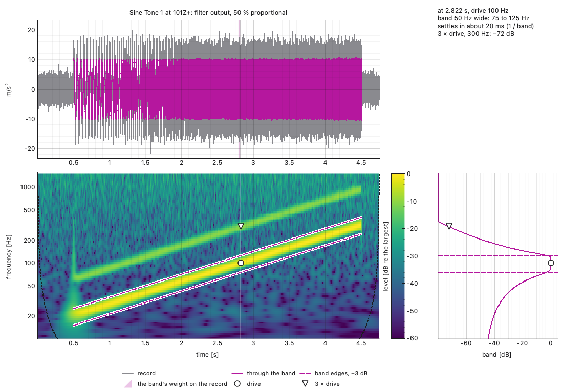
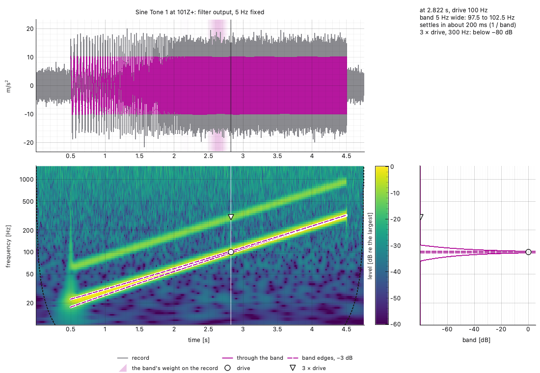
The picture's wavelet resolves frequency to about 7 % either side of the tone, so a band narrower than that, such as a 10 % proportional band or a few hertz fixed, draws as a corridor inside the tone's ridge. That is a limit of any picture of a moving tone, not a fault in the band. Shown in a window, the cursor can be dragged along either time axis, and the shape, the marks, the weight and the readout follow it.

In a script¶

from visualdynamics.core.sine_tracking import (SineTracking, track_sine,
                                               track_waveform)
from visualdynamics.plot import plot_sine_tracking, plot_tracking_filter

settings = [SineTracking(detector='peak'),          # no band
            SineTracking(proportional=0.5),          # 50 % of the drive
            SineTracking(proportional=0.1),          # 10 %
            SineTracking(fixed=10.0, detector='rms')]

levels = track_sine(history, specification, settings)   # one SineLevel each
plot_sine_tracking(history, specification, settings, path='tracking.png')

band = SineTracking(proportional=0.5)
waveform = track_waveform(history, specification, band)  # every sample
plot_tracking_filter(history, specification, band, cursor_hz=100.0,
                     path='band.png')

track_sine reads one tone (the specification's first, or tone=) on the control channels, or on any channels named with channels=. The tone's sweep is found in the record the way the extraction finds it, or placed at onset=. Every setting is read at the same lines along the sweep, so the levels overlay line for line. Each is a SineLevel in the record's own units, stamped with the second each line was read, its comment naming the reading (SineTracking.describe()). SineTracking.settling(frequency) is the one-over-the-bandwidth rule at a given drive frequency.

track_waveform runs the same band over every sample of the tone's span and keeps the passed waveform (passed) and the band's output amplitude (level), with the drive frequency at each sample; instant(frequency) finds when the drive passes a frequency. SineTracking.response(drive, frequencies) is the band's shape in dB at a given drive frequency, and SineTracking.weighting(drive, lags) its weight on the record before an instant. plot_tracking_filter draws all of them for one setting. Its cursor is placed by cursor= in seconds or cursor_hz= in hertz, span= zooms the time axes, and harmonics= names the multiples of the drive to mark (the third by default).

The plot draws one channel, each reading in its own color and with its own marker shape, and the specification's target behind them in gray.

Where judgment lives¶

This is a reading for understanding a controller, not a better level. The extraction solves every tone jointly, debiases the amplitude and chooses its smoothing from the data; a report should use it. A tracking filter reads one tone at a time and carries whatever its band lets through.
The filter runs forward only. A controller's filter cannot see ahead, so neither does this one: the lag is the measurement. It starts settled on the tone's first cycle, as a controller's has settled during its ramp-up.
A wide fixed band at the bottom of a sweep is not about the drive frequency. Where half the band reaches past the drive frequency toward zero, the band includes everything below the drive as well, and the reading shows a ripple at twice the drive.
A peak is the peak of the samples. It reads low by at most cos(π × drive / sample rate): 0.3 % at a fortieth of the sample rate, more on a harmonic near the top of the band.
RMS and mean read the waveform between the samples. Near the top of a band a cycle can be a few samples long, and an average of the samples alone misses the span by part of a sample and the waveform's shape between them. So the two are read from the record upsampled until a cycle has 64 points, over exactly the span's phase: a clean tone reads within 0.1 % down to under three samples a cycle.
No view in the application yet. The readings and both plots are scripting calls; the window does not offer them.