Lines outside a band by chance

A comparison counts the lines of an averaged PSD that fell outside each pair of limits about the specification. Some of those lines are the test, and some are the average: every line of an averaged PSD scatters about its true level by an amount its degrees of freedom set (What an average is worth), so even a response whose true level sits exactly on the specification puts some lines outside a narrow band. The Chance reading of a comparison sets beside each count the number of lines chance alone would put there at the comparison's degrees of freedom, so a real excursion can be told from the scatter of the estimate.

How many lines chance puts outside

An averaged autospectrum is the true one times a chi-square variable over its degrees of freedom. So with the true level on the target, the share of lines reading outside a band depends on nothing but the band's width in decibels and the degrees of freedom:

Degrees of freedom	Outside ±1.5 dB	Of them, low	Outside ±3 dB
50	8.8 %	5.9 %	0.13 %
100	1.6 %	1.2 %	0.0007 %
120	0.85 %	0.65 %	0.0001 %
200	0.072 %	0.062 %	0.00000004 %

On a 400-line comparison at 120 degrees of freedom, three or four lines are outside a ±1.5 dB band on any one average, in different places on the next, and a line outside ±3 dB is all but certain to be real. Most of the chance misses are low, because an average reads further below the truth than above it. A band narrower than the degrees of freedom can hold is a statement about the statistics: it shows lines outside on every run.

The expected count is the sum, over the lines judged, of each line's chance of reading past each edge, at that line's edges in decibels from the target. A count near its expectation is the scatter. A count well above it, from a group of adjacent lines on one side of the target in the same place average after average, is a real excursion.

Combining lines

Some test documents allow adjacent control lines to be combined for judging a tolerance. The powers of N adjacent lines are added into one wider band and judged against the limits' power over the same band. The sum is worth more degrees of freedom than one line, so the chance scatter shrinks while an excursion that holds across neighboring lines survives. The combination changes how the test is judged, not the test, and is agreed before it.

How much more the sum is worth depends on the window. A window spreads each line's power into its neighbors, so the estimates at adjacent lines vary together: not at all under a rectangle without overlap, and by 0.44 at one line apart under a Hann window. The PSD carries this correlation from the averaging it was computed with (Psd.line_correlation, from core.averaging.line_correlation), and a group's degrees of freedom are those of a sum of correlated estimates,

(sum of a_i)**2 n / (sum over i, j of a_i a_j r(|i - j|))

where a_i is the power the target asks of each line, n a line's degrees of freedom and r the correlation between lines that far apart. With no correlation it is Satterthwaite's, exactly N times a line's on a flat stretch and a little less where the target slopes across a group, because the louder lines carry more of the sum. Under a Hann window, the default, eight lines averaged over sixty half-overlapped frames are worth 488 degrees of freedom, not the 910 that eight lines of 113.8 would add to, and white noise averaged that way measures the same; read as independent, a narrow band would see about five times the groups outside that chance predicted. The same holds for a cell of a specification coarser than the lines, which is a sum of the lines under it. A PSD that does not carry its correlation (one read from a file without it) has its summed lines taken as independent, and the result says so in a note. A group does not reach across a stretch the specification leaves unwritten, and the last group of a stretch may hold fewer lines.

In the app

Select a specification and the PSD measured against it, and choose Chance on the plot bar, beside Spectra, RMS Error and Lines Out. The plot shows one channel, the one picked in the table under the plot or named in the drop-down: each line's level over the target in decibels, the target at zero, the warning edges dashed and the abort edges solid. Each line outside is marked with a triangle pointing the way it is out, hollow past the warning band and filled past abort. The title and the legend give each count beside its expectation.

The panel beside the plot sets Combine lines, one by default, and DOF, the degrees of freedom of one line. Left at from the PSD, the count is the one the PSD was stamped with when it was computed; a PSD read from a file does not carry one, and the reading asks for it rather than guessing. Under the settings the panel shows the degrees of freedom per line and per group, how many lines (or groups) were judged, and for each pair of limits the count outside, below and above, beside the number expected by chance. Every edit redraws the plot. The reading is recorded in the console as its plot_chance call.

From a script

import numpy as np

import visualdynamics
from visualdynamics.core.averaging import Averaging
from visualdynamics.core.chance import compare_chance, describe_chance
from visualdynamics.core.data import Specification, TimeHistory

rate = 5120.0
averaging = Averaging(frame_length=1024, overlap=0.0, window='boxcar',
                      frames=60)                  # 120 degrees of freedom
noise = np.random.default_rng(3).standard_normal(averaging.span)
history = TimeHistory(np.arange(averaging.span) / rate, noise[None],
                      response_dof=['1Z+'], ordinate_dim=['acceleration'])
history.averaging = averaging
psd = history.compute_psds()
psd.ordinate[0, (psd.abscissa >= 1200) & (psd.abscissa < 1280)] *= 10 ** 0.25

level = np.full((1, 2), 2.0 / rate)               # white noise's true level
bands = {f'{pair}_{side}': level * 10 ** (sign * db / 10)
         for pair, db in (('warning', 1.5), ('abort', 3.0))
         for side, sign in (('lower', -1), ('upper', 1))}
spec = Specification(np.array([30.0, 1970.0]), level, response_dof=['1Z+'],
                     ordinate_dim='acceleration**2/frequency', **bands)

print(describe_chance(compare_chance(spec, psd, scale_db=0), 'warning'))
# 18 of 389 lines outside the warning band (1 below, 17 above),
# 3.3 expected by chance (2.5 below, 0.8 above)
print(describe_chance(compare_chance(spec, psd, scale_db=0, combine=8),
                      'warning'))
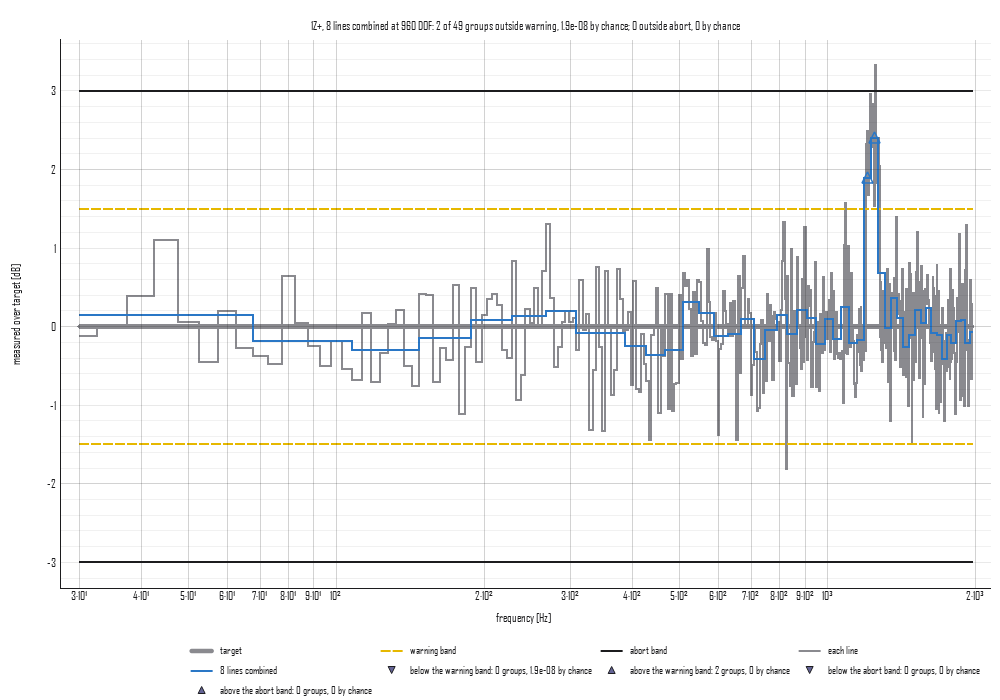
# 2 of 49 groups outside the warning band (0 below, 2 above),
# 1.9e-08 expected by chance (1.9e-08 below, 0 above)

visualdynamics.plot.plot_chance(psd, spec, combine=8, scale_db=0,
                                path='chance.png', show=False)

This is the figure: white noise averaged over sixty unwindowed frames, 120 degrees of freedom, against a flat specification at its true level with warning at ±1.5 dB and abort at ±3 dB, and sixteen adjacent lines from 1,200 Hz raised 2.5 dB as a real excursion would be. Line by line, fifteen of the sixteen are out (the scatter pulled one back in), and three chance misses elsewhere, two high and one low, against 3.3 expected; eight lines at a time, the misses are gone and the excursion is two groups out.

chance_outside(dof, lower_db, upper_db) gives the shares for one line on plain numbers, the inverse of the confidence band's chi_square_factors. compare_chance returns, beside the counts and expectations, a table of every line or group judged: its reach, its degrees of freedom, its level over the target, its edges and whether it is out. With combine 1 the counts are those compliance.compare reports.

What is refused

A pair that cannot be compared is refused as compare refuses it. A PSD on proportional bands is refused as well, since each band holds a different number of lines and so a different number of degrees of freedom; compare the narrowband spectrum. A PSD that does not say how it was averaged is refused until its degrees of freedom are given. A cross term is refused, as the confidence band refuses it: the chi-square law is an autospectrum's.