Checking a spectrum against its record

The area under an autospectral density (an ASD, in g²/Hz) is the mean square of the record it came from. That is Parseval's theorem, and it gives the cheapest check there is on a spectral computation: the sum of the lines, each times the line spacing, square-rooted,

\[ x_\text{rms} = \sqrt{\sum_k G_{xx}(f_k)\,\Delta f}, \]

should come back to the rms of the time history. A spectrum that cannot give back the rms of its own record has a scaling error in it, whatever its plot looks like, and the plot will not show it: a density read 1.76 or 3 dB high has the same shape as the right one.

The errors the check catches are few and each leaves its own gap:

• The window's amplitude correction applied to a density. A density takes the energy correction and a tone's height the amplitude correction (Reading a tone's amplitude), and their ratio is the window's noise bandwidth, so the mistake reads every line that many times too high: 1.5 for Hann, +1.76 dB.
• The one-sided doubling left out (a two-sided density, −3.01 dB) or applied twice (+3.01 dB).
• One side in g and the other in m/s², ±19.83 dB.

With no window and frames laid end to end, every sample is used once at the same weight and the two rms agree to rounding. A tapering window weights the middle of each frame more than its ends, so a windowed average is an estimate of the record's mean square rather than an identity, and on a long random record it lands within a few hundredths of a decibel. The default threshold is 0.05 dB for that reason.

A shorter or narrower record scatters further, most of all under Hann frames laid end to end, which use each frame's ends hardly at all. So the check also reads the mean square the frames themselves saw: each frame leveled as the averaging levels it, windowed, its mean square taken with the sum of the window's squares, and the frames averaged. A correctly scaled spectrum computed with that averaging carries exactly that, to rounding, whatever the window. When the gap to the record is over the threshold and the gap to the frames is not, the window is the whole of the gap: the check still flags it, and says the scaling is right and the window weighted the samples unequally. On a stationary random record more overlap evens that out; on a transient the gap is where the event fell in the frames, and a longer record need not narrow it.

From a script

rms_check on an autospectrum checks one record against the time history it came from. A PSD computed in a project knows its record and its averaging, so the project does it in one call:

name = project.compute_psds('Run')
check = project.rms_check(name)
check.spectrum_rms / 9.80665         # 8.895 g rms, from the area
check.time_rms / 9.80665             # 8.899 g rms, from the record
check.gap_db                         # -0.005 dB
check.passed                         # True, within 0.05 dB
print(check.describe('g', 1 / 9.80665))
# 8.895 g rms from the spectrum, 8.899 g rms from the time history,
# -0.005 dB: agree within 0.05 dB: the spectrum carries the record's
# mean square

visualdynamics.plot.plot_rms_check(
    project[name], project['Run'], averaging=project.averaging_of(name),
    path='rms_check.png')

An imported spectrum, a controller's for instance, names the record to check it against: project.rms_check('Controller ASD', history='Run'), or asd.rms_check(history, averaging=...) on the objects themselves, where the averaging is the one the spectrum was made with when it is known (the record's own by default). The threshold is an argument, threshold_db=, for a procedure that names its own figure. The values are stored in SI, as every record is, so the rms come back in m/s² for an acceleration; describe takes the display unit and its factor. On bare arrays, visualdynamics.core.rms_check.rms_check(frequencies, density, samples) does the same.

The result is an RmsCheck:

• spectrum_rms and time_rms, the two numbers, and gap_db, the spectrum's over the record's in dB, positive when the spectrum reads high;
• framed_rms, the frames' own, with framed_gap_db (near zero for a right spectrum) and window_gap_db (the window's share of the gap), when the averaging is known and gives the spectrum's line spacing;
• passed, explained (a flagged gap that is the window's alone), cause (the scaling error a gap matches, in words) and verdict;
• the lines summed and their spacing, the samples read, the span on the record's clock, the window and its noise bandwidth, coverage (the part of the record's band the lines cover, when it is not all of it), and notes.

The frames are the ones compute_psds averages, cut, leveled and windowed by the same code, and the channel is the one it groups them by: the DOF, the quantity and, for a record with no declared units, its hint, so an acceleration and a force at one DOF are never pooled. A spectrum with no declared units and no hint, against a record with two such channels at its DOF, is refused rather than guessed at. The record's rms is read over the span the frames cover, from the averaging's start to the end of its last frame, with every capture of the channel pooled as the average pools them. Frames leveled before their window (the averaging's detrend) have the span leveled the same way, and the notes say so.

Lines that are not finite or are below zero are left out of the area, and samples that are not finite out of the record's rms (the rule the time statistics read a record by); the notes count both. A spectrum whose lines do not run from 0 to half the sample rate, such as a controller's 10 to 1000 Hz, holds only part of the record's power: coverage says which part, the verdict says the gap is not a test of the scaling, and no cause is named.

A record that is zero over the span, one with no finite sample, a spectrum whose lines are all zero, and one with no finite line (a single sample that is not finite in a frame makes every line of that frame's spectrum so) leave no gap to judge: passed is False, the verdict says which of the four it is, and the plot's heading reads "not judged". A correctly scaled spectrum is never given a cause. On white noise under the default window (Hann, frames end to end), 8 s at 2048 samples a second, about a quarter of correct spectra read over 0.05 dB and are said to be the window's gap; at 60 s about one in a hundred do.

plot_rms_check draws the spectrum with the check written in its corner: the judgment in bold ("agree", "the window's gap", "flagged" or "not judged"), both rms in the display unit, the gap against its threshold, the window's share when it bears on the verdict, and the verdict in words.

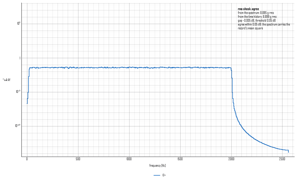
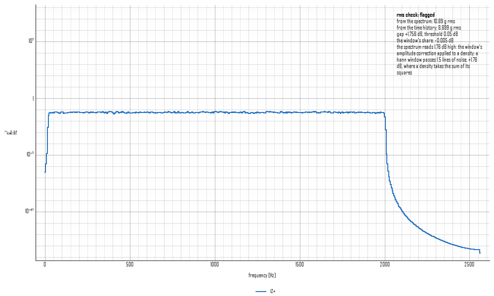
The two figures are twelve seconds of noise at 5120 samples a second, flat at 0.04 g²/Hz from 20 to 2000 Hz, averaged in 1024-sample frames under Hann at half overlap (tools/make_concept_figures.py). As the package computes it, the spectrum reads 8.895 g rms against the record's 8.899, 0.005 dB under. With every line multiplied by 1.5, the Hann amplitude correction applied to a density, it reads 10.89 g rms, 1.76 dB high, and the check names the error.

In the app

Select a PSD and press RMS Check on the bar. It is offered for an autospectrum on evenly spaced lines when the project holds a time history with its channel; not for octave bands, a cross spectrum or a record. The plot's corner carries the judgment and the gap, and the pane beside the plot shows the rest: the channel, the rms from the spectrum and from the time history, the gap, the frames' rms and the window's share, the lines, the span read and the window, with the verdict in words under them and any notes. The status line says the same in one line.

The time history is the one the PSD was computed from (marked "computed from" in the pane), checked over the frames the PSD was made with even if the record's averaging has moved since. Any other record holding the same channel can be chosen instead, which is how an imported spectrum is checked against its run. The threshold is set in the pane. Both choices are kept for that PSD. The check is of one record, the first on the plot: pick a channel in the tree to check another. While the check is up the plot stays flat. A channel of more than a million samples is checked with the progress bar up, as a long computation is.

The check is journaled as the plot_rms_check call that draws it.