The two transmissibilities, and what H1 is worth

Transmissibility is the motion at one point over the motion at another, a response over an input, at each frequency. From random data it is computed two ways, and both are commonly labeled transmissibility. They agree where the measurement is clean and differ where it is not, so a plot should say which one it shows.

The ASD ratio divides the response's autospectrum by the input's and takes the root, because an ASD is a squared quantity:

\[ T_\text{ASD}(f) = \sqrt{\frac{G_{yy}(f)}{G_{xx}(f)}} \]

It needs nothing but the two ASDs, so any two plots can be divided. It gives a magnitude and nothing else, and it has no way to tell how much of \(G_{yy}\) the input caused: whatever is on the response channel that the input did not cause (the sensor's noise floor, a rattle, a cable beating against the article, another source) is in \(G_{yy}\), and the ratio counts it as response.

H1 divides the cross-spectrum by the input's autospectrum:

\[ H_1(f) = \frac{G_{xy}(f)}{G_{xx}(f)}, \qquad \gamma^2(f) = \frac{|G_{xy}(f)|^2}{G_{xx}(f)\,G_{yy}(f)} \]

The cross-spectrum keeps the phase between the two channels and averages toward zero whatever in the response is unrelated to the input, so H1 is not lifted by uncorrelated noise on the response. The coherence \(\gamma^2\) says what share of the response at each line the input accounts for. The three are tied exactly:

\[ T_\text{ASD} = \frac{|H_1|}{\sqrt{\gamma^2}} \]

so the ratio always reads at or over H1, by \(-10\log_{10}\gamma^2\) decibels: 1.4 dB at a coherence of 0.73, 4.1 dB at 0.39. The gap says the coherence is under one. It does not say which of the two is nearer the truth; that depends on where the content the input did not cause is:

• On the response (a noise floor, a rattle, another source), H1 is unbiased and the ratio reads high, by \(1/\sqrt{\gamma^2}\).
• On the input channel (the input sensor's own noise), H1 reads low, by \(\gamma^2\), and the ratio low by \(\sqrt{\gamma^2}\), so the ratio is the nearer of the two. With the survey below's noise moved to its input channel, at 6 g rms, the truth at 1,000 Hz is 0.100, H1 reads 0.073 and the ratio 0.084, 1.2 dB above H1.
• Leakage at a sharp resonance, a nonlinearity or a second input lower the coherence as well, and bias both estimates.

The gap is \(-10 \log_{10} \gamma^2\) dB and says only that the coherence is below one; it is not a correction to apply to either curve.

What H1 is worth at a line follows from its coherence and the number of averages behind it. The normalized random error of its magnitude is

\[ \varepsilon_{|H|} = \frac{\sqrt{1-\gamma^2}}{\sqrt{\gamma^2}\,\sqrt{2n}} \]

with \(n\) the number of independent averages: 3.0 % at a coherence of 0.9 and 60 averages, 7.5 % at 0.9 and only 10. It is one standard deviation of the estimate, and a first-order result: past about 20 % it says the estimate is poor rather than how poor. The count \(n\) is what the frames are worth, not how many were cut. Overlapped frames share samples, so the error is read at the equivalent count discounted for overlap, the same discount the confidence band on an averaged PSD takes (What an average is worth); 119 Hann frames at half overlap are worth about 113.

From a script

read_transmissibility on a time history reads one response over one reference from the frames its averaging sets, the same frames compute_psds and compute_frfs use:

reading = history.read_transmissibility('101Z+', '1Z+')
reading.frames, reading.averages      # 119 frames, 112.8 independent
point = reading.at(1000.0)
point.magnitude                       # |H1|, 0.108 (the truth is 0.100)
point.asd_ratio                       # 0.126, the ratio
point.coherence                       # 0.730
point.error                           # 0.040, the random error of |H1|
point.ratio_to_h1_db                  # +1.4, the ratio to H1 in dB
print(point.describe('g/g'))
# 1000 Hz: H1 0.1077 g/g (±4.0 %, coherence 0.730); ASD ratio 0.126 g/g, +1.4 dB from H1

lower, upper = reading.band(1.0)      # |H1| (1 -+ error) at every line
visualdynamics.plot.plot_transmissibility(reading, band=(20, 1990),
                                          path='transmissibility.png')

In a project, project.read_transmissibility(frf_name, record) reads the one behind an FRF that Compute FRFs made, from the history and the averaging that FRF was computed from. Its H1 is that pair's H1 whichever estimator the FRF used. An FRF computed against several references is refused: a ratio of two autospectra would credit one input with what all of them caused.

The values are in SI, as every record is stored; for an acceleration over an acceleration that is the same number in g/g. Against a force reference the same reading is an FRF and the ratio of its spectra, not a transmissibility, and it is titled and noted that way (reading.title). A record with a sample that is not a number in the frames read is refused, naming the channel: that one sample spreads to every line of the average, and read on it would look like a line with no input power or no coherence. The same reading works on three averaged spectra as visualdynamics.core.transmissibility.read_transmissibility(frequency, gxx, gyy, gxy, frames, averages), and frf_random_error(coherence, averages) is the error expression on its own.

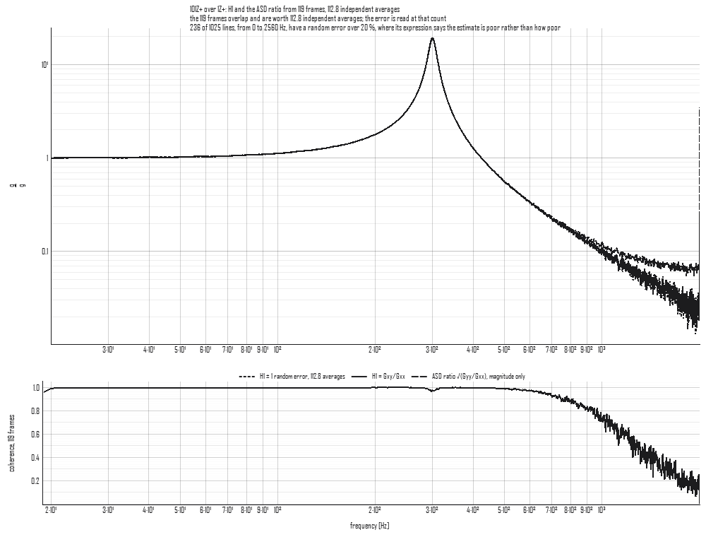
The figure is 24 seconds of random from 20 to 2000 Hz at 0.04 g²/Hz, through a 300 Hz resonance at Q 20, with 0.6 g rms of noise the input did not cause on the response channel, analyzed at 2.5 Hz lines with 119 Hann frames at half overlap (tools/make_concept_figures.py). H1 is solid, the ratio dashed and H1's band dotted, each named in the legend. Below about 600 Hz they are one curve, with a coherence near 1. Above it the response falls toward the noise: at 1,000 Hz the truth is 0.100, H1 reads 0.108 with a 4.0 % error and the ratio 0.126; at 1,500 Hz the truth is 0.043, H1 reads 0.047 with an 8.3 % error and the ratio 0.075, 4.1 dB over. The noise here is on the response, so the ratio reads high wherever the coherence is low, and H1 scatters about the truth, its band saying by how much.

In the app

Select an FRF made by Compute FRFs, drawn as its magnitude, and press Transmissibility on the bar. Over the FRF the ASD ratio is drawn dashed and H1's band dotted, with a key in the corner saying which line is which. Where the FRF is Hv or H2, H1 is drawn solid beside it, since the band belongs to H1. A dashed cursor stands on the resonance; drag it anywhere. The pane beside the plot shows the reading at the cursor's line: |H1| and its phase, the ASD ratio and how far it stands from H1, the coherence, the random error and the band it gives, and the frames and the independent averages, with notes under them. The status line says the same in one line.

The button is offered only where the reading exists: an FRF whose time history is in the project, against one reference, drawn as its magnitude. An imported FRF has no autospectra behind it to divide. The reading is of one record, the first on the plot; pick a pair in the tree to read another. The reading is journaled as the plot_transmissibility call that draws it.