Checking each channel against its range

Every input measures over a window, its range, and a signal larger than the window is clipped: each sample past the edge is written as the edge, and the tops of the waveform come out flat. The averaged spectrum hides it. Clipping takes a little energy off the few peaks that cross the edge and spreads it across the band as harmonics, and over dozens of frames the spectrum ends up a fraction of a decibel low in band with a slightly raised floor above it. The kurtosis hides it too: a Gaussian record clipped at 2.8 standard deviations reads about 2.86, inside the kurtosis bars' band of 2 to 4. The overload is in the time history.

visualdynamics.core.overload reads every channel of a record against the range its channel table gives it, and plot_overload draws the reading: one channel's trace over its range, and every channel's headroom beside its kurtosis.

Where the range comes from

The level a channel clips at is the smaller of the channel table's DAQ Range (V), the input's range, and its Sensor Range (V), the sensor's own full-scale output, whichever is stated (ChannelTable.clip_ranges()). Its Sensitivity (mV/Unit) column is the chain's sensitivity in millivolts per the unit beside it. The range in that unit is

range [unit] = clip range [V] × 1000 / Sensitivity [mV/unit]

so a 10 V input on a 100 mV/g chain reads to 100 g, and a 0.5 V input on a 200 mV/g chain to 2.5 g. A row that states neither range gives its channel none, and the channel says so. Each channel of the record is matched to the table's row that names it, by its DOF and its channel type (or its DOF alone when the type is blank and the record has one channel there), the same match the roles use. A channel the table does not name, or names with no sensitivity, or in a unit of another quantity, has no range and says why; it is not judged against a guess. Two rows that name one channel give it a range only when they agree, and the check notes which rows; where they differ the channel has no range. A range can also be given directly in SI, one per channel or one for all.

What it reports

history.overload_check(table) returns an OverloadCheck, a ChannelOverload for each channel. The samples on the rail, the crest factor, the peak and the kurtosis are the time statistics of the channel read against that range, over the same span the kurtosis bars read; the check adds what a range makes of them.

Reading	What it is
full_scale	the range either way, in SI; NaN with reason saying why where there is none
rail, rail_share, rail_rate	the samples within the margin of the range (0.1 % by default), as a count, a share and a rate per second
crest	the largest excursion over the rms
headroom_db	the range over the largest excursion, in dB: 20 log10(range / peak). At or below 0 dB the range was reached
next_peak, next_headroom_db	the largest excursion scaled up by the step to the next level (step_db, 6 dB by default), and the headroom left there
beyond	samples further out than the range and its margin
note, cautions()	any note on the table rows the range came from, and that and any samples left out in words
statistics	the channel's TimeStatistics, for every other number

Three things are judged, each channel for the first that applies:

• Beyond the range. A converter cannot write a sample past its own range, so a record that holds one was not taken through the range the table states. The table's ranges or its Sensitivity are not the ones the record was made with, and every other number is against the wrong range.
• On the rail. More samples on the rail than rail_samples (none by default), as the time statistics judge it. A sample on the rail is one whose true value is not known, and the channel's data for that run is wrong.
• Reaches its range at the next level. The largest peak, scaled up by the step, reaches the range. A test is run up in steps, and each range is checked against the next level's peak before the step, not found wanting after it. Judged only where the range held, since a clipped record's peak is the range and scaled up it predicts nothing.

No headroom is asked for beyond that. How much a range should carry over its predicted peak is a choice a test procedure makes, and the procedures put no single number on it, so the headroom is reported and the step is set where the next level is. flagged, describe() and worst (the most samples on the rail, then the least headroom at the next level) read the whole check.

A channel that is zero throughout, or holds fewer than two finite samples, is not read: its infinite headroom would otherwise read as a channel well inside its range. It says why, in its row and in the check's words. Samples that are not finite are left out, as the time statistics leave them out, and each channel holding one says how many.

An example

Twelve seconds of Gaussian random, flat at 0.04 g²/Hz from 20 to 2,000 Hz and sampled at 5,120 a second, read 8.88 grms with a largest peak of 37 g. Three channels, each a 10 V input on a 400 mV/g chain, a 25 g range: the record at minus 6 dB, the record at full level through the range, and the record at minus 12 dB.

from visualdynamics.plot import plot_overload
from visualdynamics.units import SI

check = history.overload_check(project['Channels'])
low, clipped, quiet = check.channels
clipped.rail, clipped.rail_rate     # 287 samples, 0.47 %, 23.9 a second
clipped.crest                       # 2.83
clipped.statistics.kurtosis         # 2.86: inside the kurtosis bars' 2 to 4
low.headroom_db                     # 2.62 dB: 18.49 g against 25 g
low.next_peak / 9.80665             # 36.9 g at +6 dB, against 25 g
quiet.headroom_db                   # 8.64 dB, 2.62 dB at +6 dB
check.describe()   # Of 3 channels: 1 on the rail (2Z+);
                   # 1 reaches its range at +6 dB (1Z+).

plot_overload(history, project['Channels'],
              unit_system=SI.with_units(acceleration='g'),
              path='overload.png')

The clipped channel's kurtosis passes the kurtosis bars' band; its 287 samples on the rail do not. The channel at minus 6 dB is clean, and the check says it will not be at full level: the step that clipped the second channel would clip it.

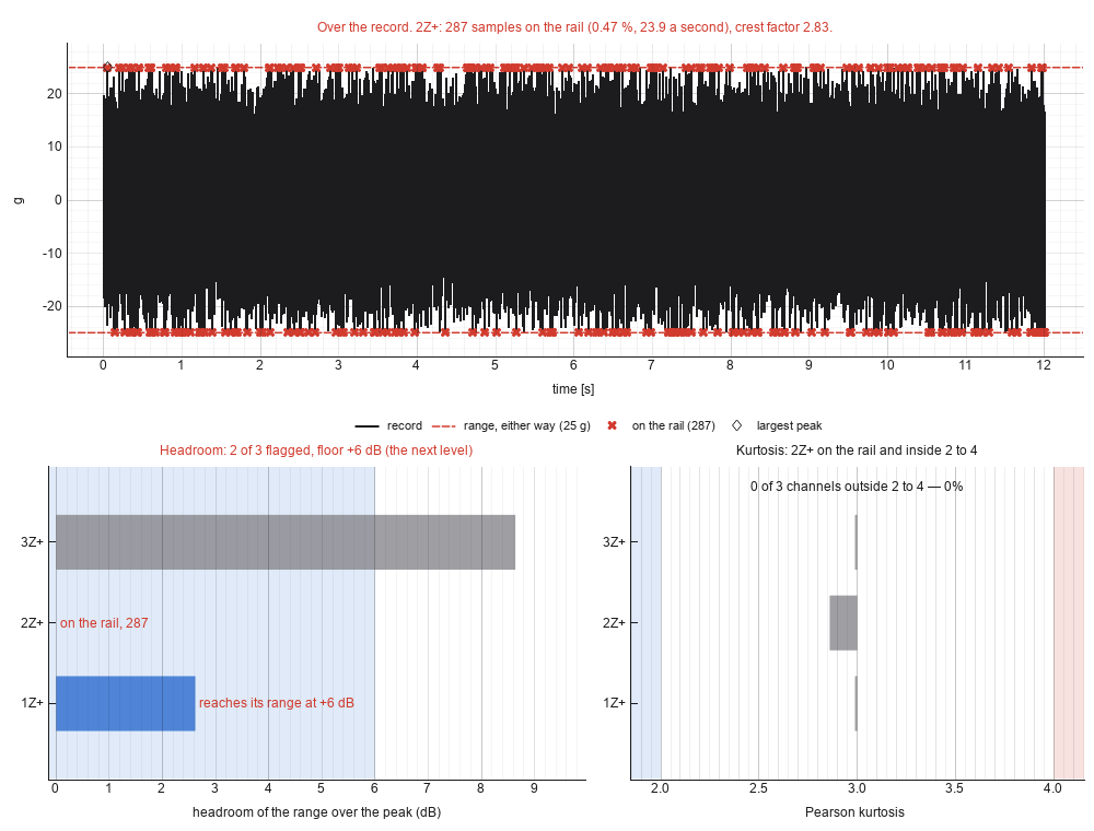
The trace is the worst channel unless record names one. Where the range held, the largest peak scaled to the next level is drawn either way as dotted lines, so the range and the peak the next step brings are seen together. The headroom bars grow from zero, with the step as a floor shaded behind them; a channel with no range has its reason written along its row instead of a bar. Nothing is told apart by color alone: the range is dashed, the next-level peak dotted, the rail samples are crosses, and every flagged bar carries its finding in words.

In the app

Overload is on a time history's bar beside Kurtosis and Statistics, one of the readings of a record, once a channel table linked with the record names one of its channels; it reads the ranges from that table. The panel names the table the ranges came from and holds the step to the next level and the margin; under them is a row a channel, its headroom and its samples on the rail, with each flagged channel in bold, then the numbers for the channel the trace draws, and the judgment in words. A channel with no range says why in its tip. Clicking a channel's row draws its trace. Dragging the floor on the headroom bars moves the step. A record of more than 300,000 samples, every channel counted, is read with the progress bar up. Every edit redraws at once, and the reading is journaled as its plot_overload call.

Where judgment lives

• The range in the table. The check is only as good as the DAQ Range, Sensor Range and Sensitivity columns, which is why a sample beyond the range is flagged as a table that does not match the record. Where the sensor's full-scale output is left blank, a sensor that clips ahead of the input leaves flat tops inside the range the input gives, and those are found by the time statistics' excursions at the peak.
• The step. The scaled peak assumes the structure behaves at the next level as it did at this one. Joints slip, resonances move and rattles wake up at full level, so the scaled peak is a starting point, never a ceiling.