Judging a multi-point control run

A random test on one shaker is often controlled at more than one point. The controller combines the control channels' spectra, line by line, into one composite and holds the composite to the reference. A run controlled this way has two results: the composite against the composite band, and each control channel against its own band, which is usually wider. This page describes how Visual Dynamics forms the composite, how it reads both results, and how to run the reading from a script.

Why there are two judgments

The control plot a controller shows is a statement about the composite. It says nothing about any one channel. Two cases show what it can hide:

• A dead channel inside an average. One of three control channels reads near zero, because its sensor has come loose or its cable is open. The controller averages it in and drives the other two up to make up the difference: each runs at one and a half times the reference, +1.8 dB, and the composite reads in tolerance at every line. Only the channel against its own band shows the fault.
• A hot spot diluted by the others. One mounting point of four rides a fixture mode at five times the response of the other three. The controller holds the average on the reference, so the hot point runs at two and a half times the reference, +4.0 dB, and the other three at half, −3.0 dB. The composite shows nothing at all; the hot point is over-tested by 4 dB and the rest under-tested by 3.

So the reading here gives both results, and for each channel it lists the lines where the channel is outside its own band while the composite is inside its band. Those are the lines the composite hides.

The strategies

The strategy says how the channels are combined. It is part of the test definition, written in the procedure and the report with the channel locations, because each one drives the table differently.

• 'average' holds the mean of the channels' densities to the reference, each counted alike. The average is taken on the densities, not on their decibels, because that is the arithmetic a controller does: one channel at four times the reference and one at a quarter average to just over twice the reference, +3.3 dB, not to 0 dB.
• 'weighted' is the average with a weight for each channel. The weights are scaled to add up to one.
• 'maximum' holds the highest channel at each line to the reference, so nothing sensed is over it and every other point is under it. The reading counts, for each channel, the lines at which it is the one the composite takes, since no single location sees the reference.
• 'minimum' holds the lowest channel at each line to the reference, so every point sensed meets it and every other point is over it.

The rule

1. The channels. The control channels are the autospectra of one measured PSD: the ones named, by record or by DOF; by default the ones at the channels the channel table flags as Control (the table in the PSD's object group in the app, table= in a script), each matched by its DOF and the quantity its row declares; and without such a table, the ones that pair with the specification's records by DOF and quantity, the same pairing the comparison uses. Two or more are needed; with one, the comparison itself is the reading, and naming none is refused as such. A channel named twice, a cross term, or a DOF that holds two autospectra (a force and an acceleration at a drive point) is refused with the reason.
2. One quantity. The channels must hold the same quantity, by the rule every comparison uses (Units in a comparison): an average of an acceleration and a velocity is refused, and so is a channel with undeclared units beside a declared one. With neither declared, the channels are combined as raw numbers and the reading says so.
3. One reference. The composite is held to one record of the specification: the only record when there is one, or the record each channel pairs with, which must all ask for the same level. A specification that asks the channels for different levels is refused unless the record to use is named.
4. The composite. At each line the strategy combines the channels' densities. A line where any channel is not a finite, non-negative number has no composite and is not judged: averaging the others there would be a composite of other channels. A channel reading zero is a reading and is counted, as a controller counts it.
5. The bands. Each band is one of the specification's pairs of limits ('warning' or 'abort'), or a pair of dB below and above the reference, ten log ten on a density. An infinite edge is no edge on that side. By default the composite is judged against the specification's warning limits and each channel against −6/+6 dB. Those are starting points to edit, not a standard: the test plan names both bands.
6. The judgment. The composite and each channel are compared with their band by compare and exceedances in visualdynamics.core.compliance, the comparison every random reading makes: cell by cell, as areas, at the comparison's one scale. A run captured below the requirement is scaled once for every channel and the composite alike.
7. The hidden lines. For each channel, the lines outside its own band at which the composite is inside its band, and judged there.

The reading also says what the reader should know about the data: the lines where a channel has no usable value, a channel that reads zero everywhere or more than 20 dB below the others at its median line (as a dead or disconnected sensor does), a weight of zero, a scale detected from the data, and units undeclared on both sides.

A reading that judged nothing says so. When one channel has no usable value at any line, the composite is formed at no line, and the composite's line reads "not judged" instead of a count of lines outside; a channel with no finite line reads the same way. Neither is ever shown as inside its band.

The bands are judged line by line, and a correct channel's spectrum scatters about its true level as much as its averaging leaves it to. For channels of white noise at the reference under the default frames (Hann, end to end), about one line in a hundred of a channel falls outside −6/+6 dB by chance with 5 frames averaged, about three in ten thousand with 10, and none with 40, and each such line is listed as a line the composite hides. A short run therefore shows a few hidden lines on channels that are working; a fault shows as many lines in a row. The dead-sensor note never trips on such channels. Where the PSD says how many degrees of freedom its averages carry and the channel band is in dB, the reading says this for the run in hand: the notes give the share of a working channel's lines that chance alone puts outside the band at that count (core.chance.chance_outside), and the status line repeats it beside the hidden lines.

In the app

Select the specification and the control PSD together. Where the measurement holds two or more control channels (the records picked, or, with the whole PSD selected, the ones that pair with the specification), Composite is on the bar beside Spectra, RMS Error, Lines Out and Chance. The plot is the picture below. The panel beside it holds the strategy, the weights under a weighted average, the composite band and the channel band, each either the specification's limits or a band in dB. Under them are the composite's lines outside its band, each channel's lines outside its own and how many of those the composite was inside at, and the notes. Every edit makes the reading again, with the progress bar up while every channel is judged (each line of each channel is judged twice, so even a short run of a few channels takes a moment), and redraws it; a redraw with nothing changed shows the reading already made. Nothing is made, so there is no Apply button; the console records the plot_multi_point call that draws what is on screen. The table under the plot still holds every channel's comparison against the specification.

In a script

from visualdynamics.core.multi_point import multi_point
from visualdynamics.plot import plot_multi_point

# the control PSD and the specification, as the random workflow makes them
reading = multi_point(spec, psds, channels=['1Z+', '2Z+', '3Z+', '4Z+'],
                      strategy='average',
                      composite_band='warning', individual_band=(-6.0, 6.0))
print(reading.outside_lines, 'lines of the composite outside',
      reading.composite_text)
for channel in reading.channels:
    print(channel.label, channel.outside_lines, 'outside its own band,',
          channel.hidden_lines, 'with the composite inside')
for note in reading.notes:
    print(note)

plot_multi_point(psds, spec, channels=['1Z+', '2Z+', '3Z+', '4Z+'],
                 path='composite.png')

reading.composite is the composite as a PSD of one record, which can be drawn or added to a project like any other. composite in the same module combines plain arrays, (channels, lines), by the same rule.

The picture

plot_multi_point draws the reference in gray, the composite band and the individual band around it shaded the way a specification's zones are (yellow between the two bands, the ground a channel may stand in and the composite may not; red above and blue below the individual band), each channel light in its own color and marker, and the composite heavy in the plot's own foreground color. Every line a channel is outside its own band is that channel's marker filled; every line the composite is outside its band is a filled circle on the composite. Each legend entry gives the count, and each channel's says how many of its lines the composite was inside at.

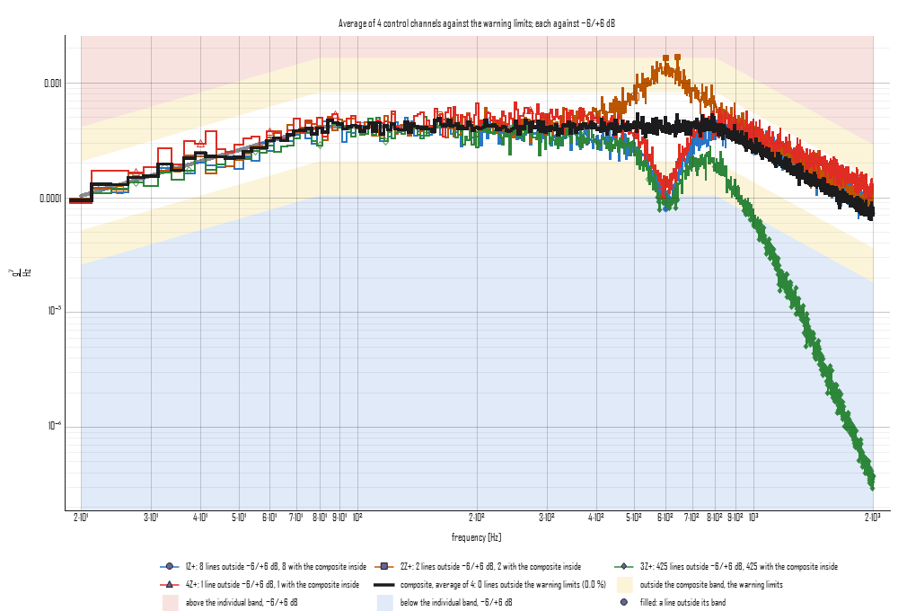
In the figure the composite is inside its band at every line. The channel through the fixture mode near 600 Hz stands between the two bands, where a channel may be and the composite may not. An average of four channels lets no channel run more than 6 dB over the composite, so under average control a hot spot is pulled back toward the reference with the others and shows only on its own channel. The channel whose reading falls away above 800 Hz, as a sensor on a cracked mount reads, is outside its own band at 425 lines, and at every one of them the composite was inside: the control plot alone would have shown nothing there.