Fatigue damage, extreme response and time compression

Two vibration environments are not compared by laying their spectra on one plot. A field record and the test written to stand for it differ in shape, in level and in duration, and what matters is what each does to the article. So both are run through the same set of single-degree-of- freedom resonators, one at each natural frequency across the band, and two numbers are read off each resonator's response:

• the extreme response spectrum (ERS), the largest response the resonator reaches over the duration: the strength question;
• the fatigue damage spectrum (FDS), the fatigue damage that response does over the duration: the life question.

A test whose ERS and FDS stand at or above the field's at every natural frequency is at least as severe, mode for mode, whatever its shape. That is how a specification is derived from field data, and how the question "is this test harder than that one" gets an answer.

The resonators and the damage

Each resonator is base-excited at natural frequency f_n and amplification Q. Its response is the relative displacement z between mass and base, the motion that strains a part, written as a pseudo-acceleration (2πf_n)²z so it reads in the input's unit. Its gain from base acceleration is

\[ H(f) = \frac{1}{1 - r^2 + j\,r/Q}, \qquad r = f/f_n , \]

one at low frequency, Q at f_n. Under a flat density G the response's mean square is exactly (π/2) f_n Q G, Miles' equation, and it crosses zero upward exactly f_n times a second.

Fatigue is read through an S-N curve, N S^b = C: a cycle of amplitude S uses S^b/C of the life, and the cycles add (the Palmgren-Miner rule). C and the stress per unit response belong to a material and a design, so they are left at one: the FDS is in the response unit to the power b, a number to compare between environments read at the same b and Q, not a life. For a response with rms σ that crosses zero ν₀ times a second, counting every crossing as a cycle of Rayleigh-distributed amplitude gives the narrow-band damage over a duration T,

\[ D = \nu_0\,T\,\bigl(\sqrt{2}\,\sigma\bigr)^b\,\Gamma\!\left(1 + \tfrac{b}{2}\right), \]

and the ERS is σ times the expected largest peak, σ√(2 ln ν₀T), the leading term of the standard result (a run usually reaches a little more).

A spectrum's cycles can be read three ways:

• narrowband, the closed form above, the default. A resonator's response is narrow-band, and for a broader one this expects more damage than rainflow counting finds, erring on the safe side.
• rice, every positive peak a cycle of its own height, the heights distributed as Rice's peaks for the response's irregularity (one for a pure tone, smaller when small peaks ride on large ones).
• dirlik, the rainflow ranges as Dirlik's empirical fit gives them from the response's spectral moments. It is a fit to simulated rainflow counts, and the package checks it against rainflow counts of simulated records.

A time history is counted directly: each resonator's response is reduced to its turning points and counted by rainflow, every closed cycle at its range, the residue as half cycles, and the ERS is the largest response in the record. Natural frequencies above a twentieth of the sample rate are refused, since a sampled response's peaks fall between samples and the damage goes as the amplitude to the power b; the result says how low its top resonator reads.

Time compression

At one exponent, a test at ASD W₁ for a time t₁ does the damage of the service level W₂ for t₂ when

\[ \frac{t_2}{t_1} = \left(\frac{W_1}{W_2}\right)^{b/2}, \]

the rule test documents give for trading time for level. The ratio W₁/W₂ is the exaggeration factor on the ASD; documents commonly cap it at 4 (2 on the rms), because a higher level can fail an article through a mechanism the exponent does not describe. The exponent is the document's convention, commonly 7.5 for random and 6 for sine, and it is never assumed here: every reading names its b. A tenfold compression at 7.5 is 1.848 on the ASD, +2.67 dB; at 4 it is +5 dB. At the cap, 7.5 allows 181 to 1 and 4 allows 16.

From a script

from visualdynamics.core.fatigue import (psd_spectra, history_spectra,
                                         compared, time_compression)

field = psd_spectra(spec, b=7.5, duration=3600.0, frequencies=[100.0])
field.rms / 9.80665          # 7.875 g: Miles' 7.93, less the band's ends
field.crossings              # 100.5 upward crossings a second
field.ers / 9.80665          # 39.84 g, expected over the hour
print(field.rests_on)        # the reading, b, Q and the peak's formula

record = history_spectra(run, b=7.5)            # counted by rainflow
pair = compared(run, test_spec, field_duration=3600.0,
                test_duration=360.0, b=7.5)     # one set of frequencies
pair.damage_db               # test over field, per natural frequency
pair.factor_needed           # on the test's ASD to cover the field
pair.duration_needed         # or the test's time at its own level
pair.exaggeration            # the factor the test carries, per frequency
print(pair.describe())

print(time_compression(b=7.5, time_ratio=10.0).describe())
# compresses time 10 to 1 at 1.848 on the ASD (+2.67 dB, 1.359 on the
# rms), b = 7.5; within the cap of 4 on the ASD

visualdynamics.plot.plot_fatigue(run, b=7.5, duration=3600.0,
                                 against=test_spec, against_duration=360.0,
                                 path='fatigue.png')

Here spec is a flat 0.04 g²/Hz from 20 to 2000 Hz. Values are in SI, as every record is; the FDS is in (m/s²)^b and the plot draws it in the display unit to the power b. fatigue_spectra(data, record, ...) takes either a PSD or a time history, and a duration given for a time history scales its FDS from the record's length, which takes the record as a stationary sample of the whole; its ERS stays the record's own. ResponseSpectra.at_duration does the same afterwards.

What cannot be read one way is refused with its cause: a record whose units are not declared, a record of another quantity than acceleration, a cross spectrum, a line or sample that is not finite (its frequency or time named), a line below zero, a spectrum with no area or a record that does not vary, a Q outside 1 to 500 or a b outside 2 to 25, and a spectrum with no duration. Two results set against each other must be read at one Q, one b and one set of natural frequencies.

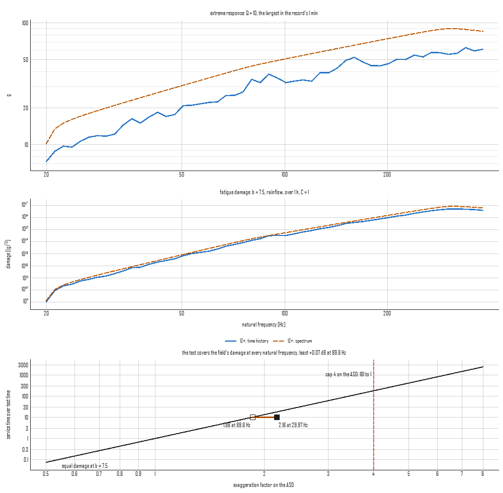
The figure (tools/make_concept_figures.py) is one minute of a vehicle floor's record, taken as a sample of an hour in service, flat at 0.02 g²/Hz from 20 to 80 Hz and 0.04 to 300 Hz then falling, set against a specification on the same breakpoints at twice the density for six minutes, at b = 7.5. A time ratio of ten wants 1.85 on the ASD and the test carries 2, so its FDS covers the field's at every natural frequency; the bar on the rule runs from the least exaggeration the test carries (the hollow square, the governing frequency, where the minute ran hardest) to the most, right of the equal-damage line and well left of the cap. The test's ERS, expected over six minutes, stands above the largest response the minute reached.

In the app

Select one acceleration record (a PSD, a specification, or one channel of a time history) and press Fatigue on the bar. The plot is the ERS, the FDS and the time-compression rule at b with its cap; the pane beside it sets the candidate test (any other acceleration record in the project), b, Q, the reading of a spectrum's cycles and the durations, and reads out what each result rests on and, with a test, the least damage margin and where, the factor and the duration that cover the field, the exaggeration against the cap and the least ERS margin. A spectrum carries no duration, so the reading waits for one and says so. A long record is counted on the window's worker, and a redraw with nothing changed draws the kept result. The reading is journaled as its plot_fatigue call.