Reading a record's time statistics

A random test is specified as a spectrum, and an autospectrum keeps only how the mean square is spread across frequency. Squaring throws away the sign, the frequency axis throws away when things happened, and the average over frames dilutes anything that happened in a few of them into all the rest. Clipping, dropouts, spikes, offsets and a loosening mount all live in what was thrown away. The time history still has them, so a record is read in the time domain before its spectrum is trusted.

visualdynamics.core.time_statistics makes that reading, one channel at a time, and judges each number against a band. plot_time_statistics draws it as three rows: the trace, its histogram against the Gaussian, and its kurtosis frame by frame.

What it reports

history.time_statistics(record) returns a TimeStatistics. Values are in SI, as the record stores them.

Reading	What it is
mean, rms, std	the offset, the rms with the offset in it (as a meter reads it), and the rms about the mean
skewness, kurtosis	the third and fourth moments over the matching power of std: 0 and 3 for a Gaussian record (Pearson's kurtosis, the kurtosis bars' own estimator)
crest, peak, peak_time, peak_sigmas	the largest excursion over the rms, the signed sample, when it was taken, and how many standard deviations from the mean it sits
at_peak	separate excursions within the margin of the record's own peak, each run of neighboring samples counted once: one for a clean Gaussian record (two in about 3 records of 100), hundreds for a clipped one
nonfinite	samples that are not finite (NaN or infinite); they are left out of every other number
rail, rail_share, headroom	with full_scale given, the samples within the margin of the channel's range, as a count and a share, and the range over the largest excursion
tails	for 3, 4 and 5 sigma, the share of samples beyond, beside the Gaussian's (0.27 %, 0.0063 % and 0.000057 %)
crossings, spectral_crossings	upward crossings of the mean per second, counted, and from the record's own spectrum by Rice's formula
bandwidth	the record's statistical bandwidth from its own spectrum, (∫G)² / ∫G²: a flat band's own width, 2πζfₙ for a single mode
expected_peak	the expected largest peak of a Gaussian process at that rate over duration, in standard deviations: √(2 ln(ν₀T))
frame_times, frame_kurtosis	the kurtosis of each frame at each frame's middle; a frame that does not vary has no kurtosis (NaN)

flags() says, statistic by statistic, which fell outside its band, flagged lists them, and describe() says it in words. The reading covers the same span the kurtosis bars read (the frames the spectra are averaged over, the shock windows, or the whole record), so the two kurtosis values always agree.

The bands

Each band is an argument, because a band is a choice a procedure makes:

Statistic	Default band	Why
kurtosis of the record	2 to 4 (kurtosis_band)	The kurtosis bars' band, set for rattles and spikes. Settable tighter, as below.
kurtosis of each frame	2 to 4 (frame_band)	A frame is short and scatters more; a spike lifts its frame far past 4, and a frame that is all dropout has no kurtosis and is outside the band.
skewness	−0.1 to 0.1 (skewness_band)	A record that leans one way: a rattle on one side, a sensor saturating in one direction.
mean	2 % of the standard deviation (offset_share)	A bias, a channel still settling, a zero shift.
crest factor	3 to 6 (crest_band)	Below 3 the peaks were cut off; a Gaussian record practically never reaches 6, and spikes do.
samples on the rail	none (rail_samples)	A sample at the edge of the range is one whose true value is not known.
excursions at the peak	two (peak_runs)	A second peak can come within the margin of the first.
samples not finite	none	A sample with no value is a fault in the record.
share beyond each sigma	within a factor of 2 of the Gaussian's (tail_ratio)	Judged only where a Gaussian would put at least ten independent values: twice the bandwidth, times the length, times the Gaussian's share.

The band of 2 to 4 does not see clipping: a Gaussian record clipped at 2.8 standard deviations reads about 2.86, inside it, and a real record at 2.86 is ordinary. That is why the rail count and the crest factor are read beside it; they are what flag a clip. A procedure that wants the kurtosis to see one as well sets kurtosis_band tighter. A whole record of tens of thousands of samples scatters only a few hundredths about 3, so 2.9 to 3.1 holds a clean record of ordinary length and flags the record clipped at 2.8; a short record scatters more and needs a wider band.

Neighboring samples of a record are not independent, and the bands are set by how many independent values the record holds, about twice its statistical bandwidth times its length, never by its sample count. That is why the peak is counted in excursions and the tails are judged in independent values. It also sets the frame: by default a frame is long enough to hold 350 bandwidth-seconds (FRAME_PRODUCT), and never shorter than 0.2 s. A 0.2 s frame of a flat 20 to 2,000 Hz record holds 396; a 20 to 200 Hz record needs frames of about 1.9 s, and a single 2 % damped mode at 100 Hz, 12.6 Hz wide, frames of about 28 s. A record shorter than one frame has no frames, and its frames are not judged. Pass frame to choose the frame yourself. Read this way, 100 clean records each of the flat profile, the 20 to 200 Hz band and the single mode were all inside every band.

The counted crossing rate needs a record sampled well above its band. At 2.56 times the top of the band, two crossings can fall between samples and the count runs about 8 % low; the rate from the spectrum does not, and it is the one the expected peak uses.

An example

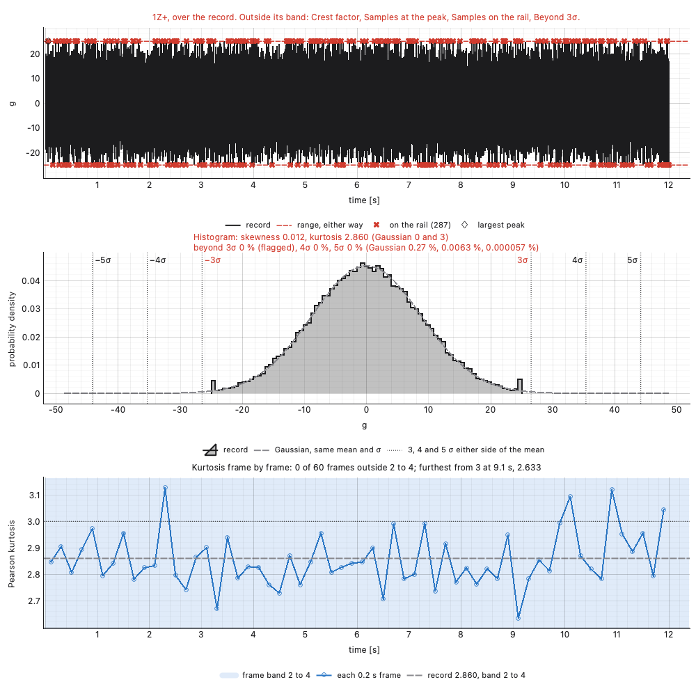
Twelve seconds of Gaussian random, flat at 0.04 g²/Hz from 20 to 2,000 Hz and sampled at 5,120 a second, read 8.88 grms with a crest factor of 4.17, a kurtosis of 2.99 and one sample at its peak. Its largest peak is 37 g. Recorded through an input ranged at 25 g, it reads:

from visualdynamics.plot import plot_time_statistics
from visualdynamics.units import SI

g = 9.80665
stats = history.time_statistics(0, full_scale=25 * g)
stats.rms / g          # 8.83
stats.crest            # 2.83
stats.kurtosis         # 2.86: inside 2 to 4
stats.rail             # 287 samples, 0.47 %, on the rail
stats.at_peak          # 278 flat tops
stats.describe()       # Outside its band: Crest factor, Excursions
                       # at the peak, Samples on the rail, Beyond 3σ.

plot_time_statistics(history, 0, full_scale=25 * g,
                     unit_system=SI.with_units(acceleration='g'),
                     path='statistics.png')

Its kurtosis passes the default band of 2 to 4, and the record is still flagged: by the samples on the rail, by a crest factor under 3, by its 278 flat tops all at its peak, and by nothing at all beyond three sigma where a Gaussian puts 0.27 %. With kurtosis_band=(2.9, 3.1) the kurtosis is flagged as well.

The expected largest peak answers a different question: how high the peaks of a run will go. At 1,000 crossings a second it is about 4.7 standard deviations for a one-minute run and 5.5 for an hour. A test's stroke, fixture and amplifier are checked at the peak the run will reach, and duration=3600 gives it for an hour from a record of any length:

from visualdynamics.core.time_statistics import (expected_largest_peak,
                                                 rice_rate)

expected_largest_peak(1000, 60)       # 4.69
expected_largest_peak(1000, 3600)     # 5.49
rice_rate(frequencies, levels)        # 1160 for the flat 20-2000 Hz profile
history.time_statistics(0, duration=3600).expected_peak

In the app

Statistics is on a time history's bar beside Kurtosis, one of the readings of a record. It reads the first selected channel and settles the tree onto it. The panel beside the rows holds the range (in the units the trace is drawn in), the margin, the frame (from band at its lowest), the duration the expected peak is for and the kurtosis band; under them is the table of every number, with each statistic outside its band set in bold, and the judgement in words under the table. Every edit redraws at once. The reading is journaled as its plot_time_statistics call.

Where judgment lives

• What the record is. The bands assume a record meant to be Gaussian random. A sine, a shock or a deliberately non-Gaussian field record is flagged by most of them, correctly and uselessly.
• The range. The rail is only counted when the range is given, and the range belongs to the input that recorded the channel, in the channel's own units. The Overload reading takes every channel's range from a linked channel table at once (checking each channel against its range).
• A flagged frame. The frame band says where to look, not what happened there. The trace at that time says what happened, a dropout or a spike or a rattle, and whether the channel is cleared or set aside.