The transformation to a point, and where the rigid body holds

A test that controls the motion of a point measures it somewhere else: accelerometers spread over the article, each along its own direction. The matrix that turns those channels into the point's three translations and three rotations is the transformation. It decides what the controller thinks the article is doing, so it is worth reading: which channel goes in where, what comes out in what unit, how well the channels resolve the six motions, and how much of what they measure the six motions leave unexplained.

A Transformation is that matrix as an object. It maps inputs to outputs, \(y = T u\), with every input and output named by its DOF and known to be a translation or a rotation.

Built from geometry, it is the pseudo-inverse of the six rigid-body shapes about the point at the input DOFs,

\[ T = \Phi^+, \qquad \Phi_{j\cdot} = \begin{bmatrix} d_j^\mathsf{T} & (e_x \times r_j)\cdot d_j & (e_y \times r_j)\cdot d_j & (e_z \times r_j)\cdot d_j \end{bmatrix} \]

for a channel along \(d_j\) at \(r_j\) from the point: the least-squares fit of six motions to the channels. It is the same matrix Transform to Modal Responses applies through a rigid set, and the one the Shape Values table shows as the response transformation.

Typed, it is whatever matrix a controller holds, with its inputs and outputs named. A virtual point is a node of its own (1000X+ … 1000RZ+), and the direction says which outputs are rotations. A controller run's matrices are already on the channel table, one per environment (The channel table): each has a column per control channel, headed by the channel's DOF, and its rows numbered, because the run's file does not name them. Name the rows and the matrix is a typed transformation, read like any other.

The units follow from the kinds. An entry joining two translations is a plain number, a rotation from translations is per length, and a translation from a rotation is a length. Values are stored in SI like everything else, and a matrix typed per inch is converted when it is made. An output rotation comes out in the angular form of the input's quantity: acceleration in, angular acceleration out, in rad/s², whatever length the matrix was typed in.

How well the channels resolve the motions

The conditioning is the largest singular value of the matrix over the smallest. It is how many times larger a relative error at the channels can reach the six motions. Entries in mixed units would make it depend on the length unit, so the rotations are first scaled by a length: the RMS lever arm of the channels about the point for a transformation built from geometry, one of the length unit it was typed in for a typed one.

A layout with every channel nearly on one line through the point sees the rotation about that line poorly. Its matrix has full rank and a large conditioning, and the pseudo-inverse is refused past a conditioning of 100 (MAX_CONDITION) unless a larger limit is asked for with max_condition, so the poor layout is found before the test and not after it. Five triaxial points on a 600 by 400 mm plate, the example below, condition at 1.79. The inverse, the six motions carried back out to the channels, is checked the same way.

What the six motions leave

With \(Q = T^+T\), the projector onto the motions the outputs describe, and \(P = I - Q\), a cross-spectral matrix at the channels splits into the part the outputs explain and the residual:

\[ G = QGQ + PGP + QGP + PGQ, \qquad \operatorname{tr} G = \operatorname{tr}(QGQ) + \operatorname{tr}(PGP) \]

The cross terms carry no power because \(PQ = 0\). For a rigid-body transformation the residual is the motion that is not rigid: the article flexing, a channel on a part that moves on its own, a loose mount, or a channel wired to the wrong DOF. Its share of the measured power, line by line, says up to what frequency the rigid-body assumption holds. The reading names the highest frequency up to which the share stays under a threshold, a tenth of the power unless another is given.

A square, invertible transformation (six channels for six motions) explains everything it is given, so its residual is zero by construction and says nothing; the reading says so. The residual needs more channels than motions.

From a script

from visualdynamics.core.transformation import Transformation

t = Transformation.from_geometry(geometry, (0.0, 0.0, 0.0),
                                 rigid.coordinate)
t.describe()        # '15 inputs to 6 outputs, conditioning 1.79, ...'
t.singular_values   # 0.657 down to 0.366
t.length_scale      # 0.264 m, the RMS lever arm
headings, rows = t.table('mm')     # per mm in the rotation rows

modal, report = t.apply(history)   # or a CPSD, or a specification
back = t.inverse()                 # the six motions out to the channels

reading = t.read_residual(history.compute_cpsds())
reading.describe()  # 'residual 66.2% of the measured power; under 10% up to 236 Hz'
reading.holds_to    # 236.0
reading.worst_channel               # '105Z+', the plate's middle point

typed = Transformation.typed(
    [[0.5, 0.5], [-0.05, 0.05]], ['1Z+', '2Z+'],
    ['1000Z+', '1000RY+'], length_unit='in')
typed.condition     # 10.0: the half-span in inches

view = project.channel_table.transformation('Random')   # a loop's matrix
loop = Transformation.typed(view.values, view.columns,  # columns: the controls
                            ['1000Z+', '1000RY+'], length_unit='in')

apply takes a time history or spectrum row by row and a cross-spectral density or specification as \(T G T^\mathsf{T}\), with a specification's bands carried where every channel wears the same one. Every input must be present, in declared units, as the quantity its kind asks for; a missing channel, a channel in undefined units, an angular record where a translation belongs, or a sample that is not a number is refused by name, and a record holding two motions at the inputs asks which (quantity=). An FRF is refused: its references transform by the force rule, which transform.to_modal applies. In a project, project.transformation_of(shapes, dofs) builds one from a rigid set at a list of DOFs or a channel table's channels, and project.read_transformation(name) reads the residual behind a density made by Transform to Modal Responses, with the conditioning reported rather than refused. t.matrix_at() draws the weights on the geometry as arrows (viz.geometry.plot_transformation), and plot_transformation_residual(reading) draws the figure below.

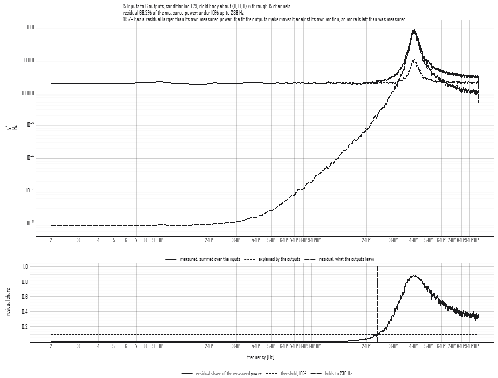
The figure is a plate measured triaxially at its four corners and its middle, moving as a rigid body under white noise, with a flexible mode at 400 Hz (Q 10) that lifts the corners and drops the middle, and a small noise floor on every channel (tools/make_concept_figures.py). The measured power is solid, the part the six motions explain dotted and the residual dashed. At 100 Hz the residual is 0.2 % of the power; it reaches the 10 % threshold at 236 Hz, 35 % at 300 Hz and 88 % at the mode. The middle point's Z channel has the largest residual of its own, 1.39 times its measured power over the band: the mode moves it down while the corners go up, and the rigid fit lifts it with the corners, so what is left at that channel is more than was measured there. The reading says so in its notes. Channel by channel, the explained part and the residual are each read on their own diagonal and need not add up to the channel's autospectrum; summed over the channels, they do.

In the app

Select a density that Transform to Modal Responses made from a CPSD through six unscaled rigid-body shapes, and press Rigid-Body Residual on the bar. The figure above is drawn in its place, and the pane beside it reads the channels and motions, the conditioning and singular values, the length scale in the display unit, the residual over the band, the frequency it holds to at the threshold and the channel with the largest residual of its own. A conditioning past the limit is said in the pane's notes. The view is journaled as its plot_transformation_residual call.