Reading a tone off an ASD

A sine tone riding on a random floor shows on the averaged autospectrum (the ASD, in g²/Hz) as a spike. The spike's height is not the tone. An ASD is a density, mean square per hertz: a broadband floor has mean square in every slice of its band, so it reads the same however finely the band is cut into lines, but a tone has all of its mean square, \(A^2/2\) for an amplitude \(A\), at one frequency, and the analysis spreads that over the lines its window leaks it into. The tallest of them stands about

\[ G_{\text{spike}} \approx \frac{A^2/2}{B_w\,\Delta f} \]

over the floor, where \(\Delta f\) is the line spacing and \(B_w\) the window's equivalent noise bandwidth in lines: 1 for a rectangle, 1.5 for Hann, 3.77 for the flat top. Analyze the same record at four times the spacing and the spike stands a quarter as tall, with the tone and the floor unchanged. It also stands lower when the tone falls between two lines than when it falls on one: by up to 1.4 dB under Hann and 3.9 dB under a rectangle. So the height of a spike says as much about the analysis as about the tone, and it cannot be compared with a tone table written in g peak.

The tone can be read off the same spectrum by summing rather than by height. The lines of an autospectrum times their spacing add up to the mean square, under any window, so the lines the tone leaks into, less the floor beneath them, times the spacing, are the tone's mean square at any spacing. Its root times \(\sqrt{2}\) is the tone in g peak.

From a script

read_tone on an autospectrum reads the tone nearest a frequency on one record, given the window the spectrum was averaged with. A PSD computed in a project has its averaging in its provenance:

name = project.compute_psds('Run')
asd = project[name]
reading = asd.read_tone(19.44, window=project.averaging_of(name))
reading.amplitude / 9.80665          # 1.942, the tone in g peak
reading.spike / 9.80665 ** 2         # 0.978, the spike in g²/Hz
reading.on_line / 9.80665 ** 2       # 1.258, its height were it on a line
reading.offset                       # 0.44 of a line off the nearest
print(reading.describe('g', 1 / 9.80665))
# 19.44 Hz: 1.94 g peak; its spike 0.978 g²/Hz (1.26 on a line) is not the tone

visualdynamics.plot.plot_tone_readout(
    asd, [4.86, 19.44, 58.32], window=project.averaging_of(name),
    snap=False, band=(2, 200), path='tones.png')

The values are stored in SI, as every record is, so the amplitude comes back in m/s² for an acceleration; describe takes the display unit and its factor. The same reading works on any evenly spaced density as visualdynamics.core.tone_readout.read_tone(frequencies, density, frequency, window=...), and returns a ToneReading: the tone's amplitude, mean square and frequency as read between lines, the spike as measured, the height this tone stands at for the spacing and window (height, over the floor), the floor, the spacing, the window's noise bandwidth, the lines summed, and any notes. spike_height(A, df, window, offset=...) and noise_bandwidth(window) are the arithmetic on their own.

How the reading is made:

1. The window's leakage, the share of a tone each line receives as a function of where the tone sits between lines, is worked out from the window's own shape. It gives the noise bandwidth and the main lobe's half-width (two lines for Hann).
2. The tone's line is the tallest within the main lobe of the frequency asked, and where the tone sits between lines is fitted from the lines about it. With snap=False the tone is taken to be at the frequency given, as a tone table states it.
3. The floor is the median of the lines either side, beyond the main lobe and a guard as wide again, with any other tone among them left out.
4. The lines within the main lobe, less the floor, times the spacing, divided by the share of the tone those lines hold, are the tone's mean square. Under Hann the lines hold over 99 % of it; under a rectangle, with the tone midway between lines, 81 %.

plot_tone_readout draws the spectrum with each tone on it: a stem from the floor up to the height this tone stands at for the spacing and window in use, a triangle on top, a dotted line at the floor across the lines summed, and the amplitude in words beside it with the spike's height under it. The triangle lands on the spike's top when the reading is right, which is how a reading taken off the wrong spike, or a floor misjudged, shows itself.

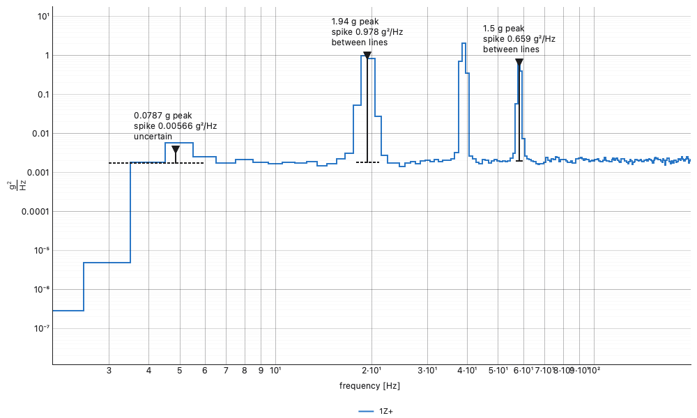
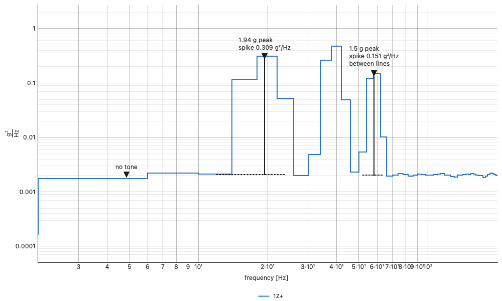
The two figures are one minute of a 1 grms floor from 5 to 500 Hz with tones of 0.12, 1.944, 2.5 and 1.5 g peak at 4.86, 19.44, 38.88 and 58.32 Hz, averaged under Hann at half overlap, at 1 Hz lines and at 4 Hz lines (tools/make_concept_figures.py). The 1.944 g tone's spike reads 0.978 g²/Hz at 1 Hz lines and 0.309 at 4 Hz, a ratio of 3.2 where the spacing alone would give 4: at 1 Hz spacing the tone sits 0.44 of a line from the nearest line, which costs its spike a fifth of its height. Its amplitude reads 1.942 and 1.943 g peak. The 0.12 g tone at the floor's lower edge reads 0.079 g at 1 Hz lines and is called uncertain, since there is no floor under it on one side to take away; at 4 Hz lines it stands no higher than the floor and reads as no tone.

In the app

Select a PSD and press Tones on the bar. A dashed cursor stands on the tallest spike; drag it to any other. Wherever it stands, the tone nearest it is read and drawn on the plot, and the pane beside the plot shows the reading: the tone in g peak and g rms, the spike's height and the height it would have on a line, the floor, the line spacing, the window and its noise bandwidth, and how far the tone sits off its line, with the notes under them. The status line says the same in one line.

The window is the one the PSD's averaging recorded when the PSD was computed (the pane says "the averaging"). A PSD that was imported carries none, and is read as Hann, the pane saying "assumed". Another window can be chosen in the pane, with its alpha or beta for a Tukey or Kaiser window, and the tone is read again under it; the choice is kept for that PSD. The reading is of one record, the first on the plot: pick a channel in the tree to read another. While the tones are read the plot stays flat, because the cursor works on the flat spectrum's lines.

The reading is journaled as the plot_tone_readout call that draws it, at the tone the cursor last read.

What is said rather than hidden

Each note is warned as a ToneWarning from a script and listed in the pane, and a reading whose amplitude it bears on is marked uncertain (the plot's words say so):

• A tone between lines. Its spike reads short, by the share the note gives. The amplitude does not move, so this one leaves the reading certain; the plot says "between lines".
• A tone at the edge of the floor's band. A line beside the tone reads far under the floor, so there is no floor under the tone to take away.
• A floor that differs either side. The floor under the tone is a guess between the two.
• Another spike among the tone's lines. Two tones closer than the window's main lobe are summed together. Finer lines or a narrower window part them; under the flat top at 4 Hz lines, tones 19.44 Hz apart cannot be parted.
• Nothing standing clear of the floor. No tone, or one too small for this spacing: the 0.12 g tone above at 4 Hz lines.
• Lines that hold no number. A line of the record that is not a number is read as zero, and one among the tone's lines or its floor's makes the reading uncertain. A record with no number in it is not read at all.

A note that names a density gives it in the units the reading is shown in: SI from a script, as the spectrum is stored, and the display units in the pane.