Predicting the drives before the test

A random test is controlled on spectra, and the controller's first drive comes from the plant it measured at low level and the profile it was asked for. The same arithmetic, done at the desk with the measured FRF and the specification, says before the article goes on the table whether the amplifiers and shakers can play the profile, which one runs out first and at what frequency, and where the profile cannot be made at all. visualdynamics.core.drive_prediction makes that prediction, for one drive or several.

It is a prediction and not a control loop. It is made once, open loop: what the first drive would be with this FRF as the plant, before any correction.

The arithmetic

The control channels' spectral density matrix is the drives' passed through the plant,

S_yy = conj(H) S_vv H^T

at every line: H the FRF matrix from the drives to the control channels (a row per channel, a column per drive, in g/V), S_vv the drives' matrix, H^T the transpose of H. The conjugate sits on the left because the package stores the cross term between channels a and b as conj(X_a)·X_b, the way compute_cpsds computes it. Turned round, the drives that make a target S_ref are

S_vv = conj(Z) S_ref Z^T

with Z an inverse of H. On one drive and one channel this is the drive spectrum a controller starts from, the target over the plant squared: a plant of 2 g/V and a target of 0.04 g²/Hz need 0.01 V²/Hz. With several drives, H is a matrix at every line, and where two drives reach the control channels in nearly the same proportions its inverse is made of noise. The inverse is regularized in one of two stated ways:

• Truncated (the default): at each line, the singular values of H under tolerance times that line's largest are dropped. The default tolerance, 0.01, drops the directions a condition number over 100 makes. On one drive nothing is ever dropped.
• Tikhonov: Z = (H^H H + λI)^-1 H^H, with λ the stated weight times the largest squared singular value anywhere in the band. Where the plant responds well this is the inverse; where it barely responds the inverse stays small. On one channel it is H* / (|H|² + λ). It pulls every line a little, by σ² / (σ² + λ) on each singular value σ, so a weight that is large against the plant's weakest gains leaves the whole band short.

A regularized inverse no longer meets the target everywhere. The prediction carries the control channels' own response to the drives it predicts, conj(H) S_vv H^T, and the lines where an autospectrum misses the target by more than 1 dB (UNMET_DB) are named. Those are the lines the inverse gave up; the cross terms are the matrix comparison's business, not this reading's.

What it reports

predict_drives(frf, specification, ...) returns a DrivePrediction. The FRF is from the drives (volts, or force for a force-controlled drive) to the control channels and to any other channel measured against the same drives; the specification names the control channels, a full cross-spectral matrix when there are several and an autospectrum when there is one. Every channel the FRF holds is predicted, so a force gauge or an accelerometer on the article comes out beside the control channels.

Each quantity is Gaussian random with a predicted autospectrum, so its rms is the root of the area under it and its expected largest peak over a run of duration seconds (a minute by default) is the rms times sqrt(2 ln(2 ν₀ T)), with ν₀ its own crossing rate by Rice's formula, from the time statistics: the largest peak of either sign, since a limit or a stroke each way is reached by either. A stated peak_factor replaces that, for a controller that clips its drive at a set multiple of the rms. Each quantity is judged on its peak:

Quantity	Read from	Against
drive	each drive's autospectrum	drive_limit, in the drive's unit
force	the moving mass times the table's acceleration	the shaker's force rating
velocity	the table's acceleration autospectrum over (2πf)²	the velocity rating, with the body counted
travel each way	the same over (2πf)⁴	half the stroke, with the body counted
response	any channel of the FRF	its limits entry, in its own unit

The shaker is a ShakerRating from core.shaker, the one the stroke readout and the replication fit judge by, given once for every drive or by drive. Its table is read at the acceleration measured at the drive's own DOF, or at the one control channel of a single-input test; tables names another. An amplifier's current is read as a response: give the FRF from the drives to the current monitor and a limit at that channel of the monitor's output at the current rating.

Each demand names the line contributing most to its mean square and the band of lines holding half of it, so the reading can say what runs out first and where. first_out is the demand nearest its rating, headroom_db how far the level could rise before it reaches it, and describe() says all of it in sentences.

An example

Two shakers drive one fixture, each with 60 lb moving on a 4 Hz suspension. The fixture's first flexible mode, its two ends moving opposite, is at 400 Hz, and the amplifiers give 150 and 120 lbf per volt. The FRF runs from the two drive voltages to the two drive-point accelerations. The specification asks each drive point for 0.01 g²/Hz from 80 to 500 Hz, rolling off at 3 dB an octave to 20 and 2000 Hz, with a coherence of a quarter between the two, in phase. Each shaker is rated 2,000 lbf, a 1 in stroke and 70 in/s, and each drive may reach 10 V:

from visualdynamics.core.drive_prediction import predict_drives
from visualdynamics.core.shaker import ShakerRating
from visualdynamics.plot import plot_drive_prediction
from visualdynamics.units import to_si

rating = ShakerRating(force=float(to_si(2000.0, 'lbf')),
                      stroke=float(to_si(1.0, 'in')),
                      velocity=float(to_si(70.0, 'in/s')),
                      moving_mass=float(to_si(60.0, 'lb')))
prediction = predict_drives(frf, specification, drive_limit=10.0,
                            shakers=rating)
print('\n'.join(prediction.describe()))
plot_drive_prediction(frf, specification, drive_limit=10.0,
                      shakers=rating, path='drives.png')

Below the fixture's flexible mode the fixture moves as one piece, so the two drives reach the two control points nearly alike: the plant's condition number is 426 at 20 Hz and falls through 100 between 40 and 42 Hz. A coherence of a quarter asks the two points to move differently, and the only way to make that is the weak direction, the two drives pushing against each other through a stiff fixture. The default inverse sets that direction aside up to 40 Hz, where the autospectra come out 1.2 to 1.3 dB under the target (the reading names 20 to 40 Hz), and keeps it just above, where it costs dearly: the drives peak at 42 Hz, the second at 7.29 V rms and 32.9 V expected, 329 % of its limit. Everything else is easy. The force is 980 lbf expected, 49 % of its rating, most of it at the fixture mode; the velocity is 6 % and the travel 3 % of theirs.

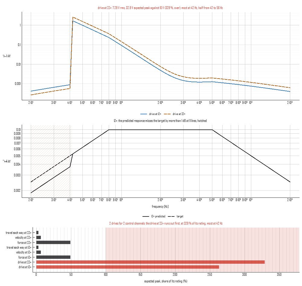
At a tolerance of 0.1 (a condition number of 10) the weak direction is set aside up to 122 Hz and through the fixture mode at 386 to 418 Hz, where the other direction is the weak one. The drives come down to 79 % and 97 % of their limit, and the target is short through those bands. That is the choice the reading puts in front of the engineer: ask the fixture for less difference between the two points at low frequency, or pay for it in drive, or accept the shortfall; none of it is a setting the controller can find on its own.

In the app

Select an FRF and a specification together and choose Drive Prediction on the bar. The plot shows the drives in line styles of their own, the first control channel predicted solid against its target dashed (or the response of the first record picked under the FRF), with the lines the inverse did not meet hatched, and a bar for every quantity judged against its rating, the one that runs out first named above it. The panel beside it takes the inverse and its tolerance or weight (only the one the inverse uses is shown), the run's duration, the drive limit and one shaker's ratings for every drive, in the window's units, zero for none; under them it says the verdict and each quantity in a line. Every edit redraws at once, the settings are kept when the selection changes, and the reading is journaled as its plot_drive_prediction call. A pair the prediction refuses (a control channel the FRF does not hold, a missing cross term, undeclared units) says why in the panel.

Where judgment lives

• The FRF is the plant at the level it was measured at. A plant that softens or stiffens with level, a fixture that rattles at full level, or an article that shifts its modes moves the drives, and the prediction knows none of it.
• The tolerance or the weight. The reading shows what each one costs, in drive and in the lines left short; which cost is acceptable is a test decision.
• The specification's cross terms. A coherence or phase the fixture cannot make is asked of the weak direction, and the reading shows the drive it takes; whether the request was meant is a question for whoever wrote it.
• The ratings and the duration. A continuous rating is the one to judge random against, and the expected peak grows, slowly, with the run.